This edition is still being built. The reference list, the symbol glossary, the acronym list and the subject index are not published yet, so some links do not lead anywhere. The twelve chapters are complete.

Parametric Uniformity and Conditional Structures

7 Reduction of C-Segments

In this chapter we will show that the conditional contribution of ca-conditionals can be generated by using only a subset of all lines within their vf truth tables. Many lines generate the same vf-pairs and therefore are redundant. Although this is obvious from looking at the vf truth tables, it is not immediately clear whether there is an algorithm which would allow finding such redundant lines. In this chapter we will introduce such an algorithm for the limited case of ca-conditionals. The mechanism is called the method of reduction of c-segments or simply reduction of c-segments, in short RCS.

The related results will be applied to c-conditionals and ca-conditionals in chapter 9. We therefore will state the propositions wherever possible in a more generic way, e.g. for atomic conditionals in general or or for cac-conditionals.
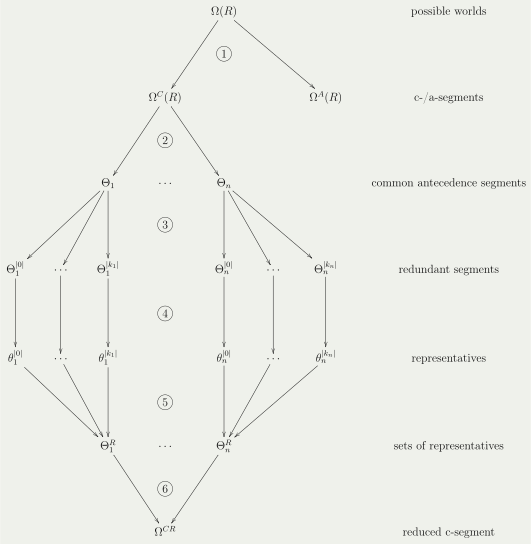
Overview of the Method of Reduction of C-Segments (RCS)
Figure 7.1 Overview of the Method of Reduction of C-Segments (RCS)

Figure 7.1 gives an overview of the steps performed in this chapter in order to define RCS. Step 1 shows the segmentation of possible worlds into c-segments and a-segments, as described already in section 4.7.

In section 7.1 we will introduce the common antecedence sets, which are the sets of c-atoms which are counted by exactly the same a-atoms of a conditional. Step 2 shows that these sets will be used to further segment the c-atoms into common antecedence segments, which will be described in section 7.2.

We will then show in section 7.3 that within a set of common antecedence segments all those segments are mutually redundant, which verify (or falsify) the same number of c-atoms (step 3). This allows us to chose only one of these mutually redundant sets as a representative (step 4). All the different representatives of one set of common antecedence segments then will be put together into a set of representatives as described in section 7.4 (step 5). We then end up with the so-called a reduced set of c-segments (step 6).

In the next chapter we will show how RCS allows us to generate the same conditional contribution as the common method (as defined by section 2.3) but in many cases with less effort.

7.1 Common Antecedence Sets

We will pave the ground in order to allow for a segmentation into redundant sets, as outlined in the previous section. For this we first have to identify the a-atoms which count the same c-atoms. These a-atoms are grouped into the countedby-set. Those c-atoms which then share the same countedby-sets form a common antecedence set.

We first define the countedby-sets.

Definition 39 (Set of A-Atoms Counting a C-atom)

Let Rcac\Rcac be a cac-conditional. Let ccat(Rcac)c\in\cat(\Rcac) be a c-atom of Rca\Rca and let gnd(Rcac)\gnd(\Rcac) be the set of groundings of Rcac\Rcac.

The set of a-atoms counting cc is

countedby(Rcac,c):={ a  <(ca)> gnd(Rcac) }. \countedby(\Rcac,c) := \{~a~|~\big<\big(c\big|a\big)\big>~\in\gnd(\Rcac)~\}.

Example 37 (Set of A-Atoms Counting a C-atom)

Continuing from example 32.

Then we get the sets of a-atoms which count the same c-atoms:

countedby(Rcac,C(a))\countedby(\Rcac,C(a))={ A(b), A(c) }= \{~A(b),~A(c)~\}
countedby(Rcac,C(b))\countedby(\Rcac,C(b))={ A(a), A(c) }= \{~A(a),~A(c)~\}
countedby(Rcac,C(c))\countedby(\Rcac,C(c))={ A(a), A(b) }= \{~A(a),~A(b)~\}

We now can define the common antecedence set as the set of c-atoms which share the same countedby-sets.

Definition 40 (Common Antecedence Set)

Let Rcac\Rcac be a cac-conditional. Let ccat(Rcac)c\in\cat(\Rcac) and aaat(Rcac)a\in\aat(\Rcac).

The common antecedence set of cc is the set of c-atoms which are all counted by exactly the same a-atoms in conditional Rcac\Rcac, i.e.

coan(Rcac, c)={ c  countedby(Rcac,c) = countedby(Rcac,c), c,ccat(Rcac) } \coan(\Rcac,~c) = \{~c'~|~\countedby(\Rcac,c)~=~\countedby(\Rcac,c'),~c,c'\in\cat(\Rcac)~\}

The following example introduces informally the common antecedence table.

Example 38 (Common Antecedence Set)

Let s1={ a, b, c }s_1 = \{~a,~b,~c~\} and s2={ x, y }s_2 = \{~x,~y~\} be sorts, V1V_1 and WW variables over s1s_1, V2V_2 a variable over s2s_2, C,AC, A predicates and Rca=< ( C(V1,V2)  A(W) ), V1W,V1c >\Rca=\big<~\big(~C(V_1, V_2)~|~A(W)~\big),~V_1\neq W, V_1\neq c~\big> a ca-conditional.

Then we get the groundings of Rca\Rca, i.e.

r1= < ( C(a,x)  A(b) ) >r_1 = ~\big<~\big(~C(a,x)~|~A(b)~\big)~\big>    ~~~~r5= < ( C(b,x)  A(a) ) >r_5 = ~\big<~\big(~C(b,x)~|~A(a)~\big)~\big>
r2= < ( C(a,x)  A(c) ) >r_2 = ~\big<~\big(~C(a,x)~|~A(c)~\big)~\big>r6= < ( C(b,x)  A(c) ) >r_6 = ~\big<~\big(~C(b,x)~|~A(c)~\big)~\big>
r3= < ( C(a,y)  A(b) ) >r_3 = ~\big<~\big(~C(a,y)~|~A(b)~\big)~\big>r7= < ( C(b,y)  A(a) ) >r_7 = ~\big<~\big(~C(b,y)~|~A(a)~\big)~\big>
r4= < ( C(a,y)  A(c) ) >r_4 = ~\big<~\big(~C(a,y)~|~A(c)~\big)~\big>r8= < ( C(b,y)  A(c) ) >r_8 = ~\big<~\big(~C(b,y)~|~A(c)~\big)~\big>

From those we can derive the sets of of a-atoms counting c-atoms:

countedby(Rca,C(a,x))\countedby(\Rca,C(a,x))={ A(b), A(c) }= \{~A(b),~A(c)~\}=countedby(Rca,C(a,y))= \countedby(\Rca,C(a,y))
countedby(Rca,C(b,x))\countedby(\Rca,C(b,x))={ A(a), A(c) }= \{~A(a),~A(c)~\}=countedby(Rca,C(b,y))= \countedby(\Rca,C(b,y))

and get the common antecedence sets:

coan1={ C(a,x), C(a,y) }\coan_1 = \{~C(a,x),~C(a,y)~\}   ~~~coan2={ C(b,x), C(b,y) }\coan_2 = \{~C(b,x),~C(b,y)~\}

Finding these identical sets is a bit complicated, at least when done manually. We therefore introduce the common antecedence table, which indicates the a-atoms as column headings and the c-segments as row headings. The cells of which the related c-atom and a-atom occur both in an admissible grounding of Rca\Rca are marked (e.g. with the indicator of the admissible grounding or simply a "*"). Table 7.1 shows such a table for this example. We see that the c-atoms of those lines, which have indicators in exactly the same columns, form a common antecedence set.

Table 7.1
A(a)A(a)A(b)A(b)A(c)A(c)
C(a,x)C(a,x)r1r_1r2r_2}coan1\Big\} \coan_1
C(a,y)C(a,y)r3r_3r4r_4
C(b,x)C(b,x)r5r_5r6r_6}coan2\Big\} \coan_2
C(b,y)C(b,y)r7r_7r8r_8
Table 7.1: Common Antecedence Table of RcacR^{cac} of Example 38

Table 7.2 shows the reduced vf truth table of Rca\Rca.

Table 7.2
coan1\coan_1coan2\coan_2
C(a,x)C(a,x)C(a,y)C(a,y)C(b,x)C(b,x)C(b,y)C(b,y)A(a)A(a)A(b)A(b)A(c)A(c)\sum
ω()a\omega^a_{()}ω(1)a\omega^a_{(1)}ω(2)a\omega^a_{(2)}ω(3)a\omega^a_{(3)}ω(1,2)a\omega^a_{(1,2)}ω(1,3)a\omega^a_{(1,3)}ω(2,3)a\omega^a_{(2,3)}ω(1,2,3)a\omega^a_{(1,2,3)}
ω()c\omega^c_{()}00000000(0,0)(0,0)(0,2)(0,2)(0,2)(0,2)(0,4)(0,4)(0,4)(0,4)(0,6)(0,6)(0,6)(0,6)(0,8)(0,8)
ω(4)c\omega^c_{(4)}00000011(0,0)(0,0)(1,1)(1,1)(0,2)(0,2)(1,3)(1,3)(1,3)(1,3)(2,4)(2,4)(1,5)(1,5)(2,6)(2,6)
ω(3)c\omega^c_{(3)}00001100(0,0)(0,0)(1,1)(1,1)(0,2)(0,2)(1,3)(1,3)(1,3)(1,3)(2,4)(2,4)(1,5)(1,5)(2,6)(2,6)
ω(3,4)c\omega^c_{(3,4)}00001111(0,0)(0,0)(2,0)(2,0)(0,2)(0,2)(2,2)(2,2)(2,2)(2,2)(4,2)(4,2)(2,4)(2,4)(4,4)(4,4)
ω(2)c\omega^c_{(2)}00110000(0,0)(0,0)(0,2)(0,2)(1,1)(1,1)(1,3)(1,3)(1,3)(1,3)(1,5)(1,5)(2,4)(2,4)(2,6)(2,6)
ω(2,4)c\omega^c_{(2,4)}00110011(0,0)(0,0)(1,1)(1,1)(1,1)(1,1)(2,2)(2,2)(2,2)(2,2)(3,3)(3,3)(3,3)(3,3)(4,4)(4,4)
ω(2,3)c\omega^c_{(2,3)}00111100(0,0)(0,0)(1,1)(1,1)(1,1)(1,1)(2,2)(2,2)(2,2)(2,2)(3,3)(3,3)(3,3)(3,3)(4,4)(4,4)
ω(2,3,4)c\omega^c_{(2,3,4)}00111111(0,0)(0,0)(2,0)(2,0)(1,1)(1,1)(3,1)(3,1)(3,1)(3,1)(5,1)(5,1)(4,2)(4,2)(6,2)(6,2)
ω(1)c\omega^c_{(1)}11000000(0,0)(0,0)(0,2)(0,2)(1,1)(1,1)(1,3)(1,3)(1,3)(1,3)(1,5)(1,5)(2,4)(2,4)(2,6)(2,6)
ω(1,4)c\omega^c_{(1,4)}11000011(0,0)(0,0)(1,1)(1,1)(1,1)(1,1)(2,2)(2,2)(2,2)(2,2)(3,3)(3,3)(3,3)(3,3)(4,4)(4,4)
ω(1,3)c\omega^c_{(1,3)}11001100(0,0)(0,0)(1,1)(1,1)(1,1)(1,1)(2,2)(2,2)(2,2)(2,2)(3,3)(3,3)(3,3)(3,3)(4,4)(4,4)
ω(1,3,4)c\omega^c_{(1,3,4)}11001111(0,0)(0,0)(2,0)(2,0)(1,1)(1,1)(3,1)(3,1)(3,1)(3,1)(5,1)(5,1)(4,2)(4,2)(6,2)(6,2)
ω(1,2)c\omega^c_{(1,2)}11110000(0,0)(0,0)(0,2)(0,2)(2,0)(2,0)(2,2)(2,2)(2,2)(2,2)(2,4)(2,4)(4,2)(4,2)(4,4)(4,4)
ω(1,2,4)c\omega^c_{(1,2,4)}11110011(0,0)(0,0)(1,1)(1,1)(2,0)(2,0)(3,1)(3,1)(3,1)(3,1)(4,2)(4,2)(5,1)(5,1)(6,2)(6,2)
ω(1,2,3)c\omega^c_{(1,2,3)}11111100(0,0)(0,0)(1,1)(1,1)(2,0)(2,0)(3,1)(3,1)(3,1)(3,1)(4,2)(4,2)(5,1)(5,1)(6,2)(6,2)
ω(1,2,3,4)c\omega^c_{(1,2,3,4)}11111111(0,0)(0,0)(2,0)(2,0)(2,0)(2,0)(4,0)(4,0)(4,0)(4,0)(6,0)(6,0)(6,0)(6,0)(8,0)(8,0)
[0][0][2][2][2][2][4][4][4][4][6][6][6][6]2[4]2[4]
Table 7.2: vf Truth Table and Common Antecedence Sets of Example 38

From this table we see that there are many redundant lines, i.e.

  • line 1 and 2, as well as 5 and 6 as well as 9 and 10 as well as 13 and 14 generate the same vf-pairs respectively;
  • the block of lines 4,5,6,7 and the the block of lines 8,9,10,11 generate the same vf-pairs.

Before we move on to the next section we state the rather obvious fact that the common antecedence sets are mutually exclusive and that they cover all c-atoms.

Proposition 17 (Common Antecedence Sets Cover Exactly All C-Atoms)

Let Rca\Rca be a ca-conditional and coan1,,coank\coan_1,\cdots,\coan_k all common antecedence sets of Rca\Rca.

It holds that cat(Rca)=i=1kcoani\cat(\Rca) = \bigcup_{i=1}^k \coan_i and for any two coani\coan_i and coank\coan_k of Rca\Rca with iki \neq k it holds that coanicoank=\coan_i \cap coan_k = \emptyset.

Proof

Based on definition 39 it is countedby(Rcac,c)={ a  <(ca)> gnd(Rcac) }{\countedby(\Rcac,c) = \{~a~|~\big<(c|a)\big>~\in\gnd(\Rcac)~\}}, so that for all ccat(Rca)c\in\cat(\Rca) there exists exactly one countedby\countedby set.

Based on definition 40 it is

coan(Rcac,c)={ c  countedby(Rcac,c) = countedby(Rcac,c), c,ccat(Rcac) }.\coan(\Rcac,c) = \{~c'~|~\countedby(\Rcac,c)~=~\countedby(\Rcac,c'),~c,c'\in\cat(\Rcac)~\}.

As all countedby\countedby sets are included in one of the coan\coan sets of Rca\Rca it follows that cat(Rca)=i=1kcoani\cat(\Rca) = \bigcup_{i=1}^k \coan_i.

As each ccat(Rca)c\in\cat(\Rca) can only be included in exactly one set countedby(Rca,c)\countedby(\Rca,c) and as all equal countedby\countedby sets contribute their c-atoms into exactly one coan\coan-set it follows that all coan\coan sets are mutually exclusive, i.e. for any tow coani\coan_i and coank\coan_k of Rca\Rca with iki \neq k it holds that coanicoank=\coan_i \cap \coan_k = \emptyset.

Example 39 (Common Antecedence Sets Cover Exactly All C-Atoms)

Continuing from example 38.

The reduced vf truth table in table 7.2 shows that coan1\coan_1 and coan2\coan_2 are not overlapping and that they cover all c-atoms.

7.2 Common Antecedence Segments

A common antecedence set is the set of those c-atoms of a ca-conditional which are all counted by exactly the same a-segment. In this section we introduce the common antecedence segments, which are based on the c-atoms in the common antecedence sets. We will show that these common antecedence segments cover all c-atoms and that they are mutually exclusive.

Definition 41 (Common Antecedence Segment)

Let Rcac\Rcac be a cac-conditional. Let coani\coan_i be a common antecedence set of Rcac\Rcac.

The set of common antecedence segments of coani\coan_i is the set of possible world segments which are based on the c-atoms of coani\coan_i and is denoted by Θi\Theta_i so that Θi=Ω(coani)\Theta_i = \Omega(\coan_i). It is θΩ(coani)\theta\in\Omega(\coan_i) a common antecedence segment.

The numbering of the indexes of the ground atoms within the common antecedence segments θ(i1,,il)Θi\theta_{(i_1,\cdots,i_l)}\in\Theta_i is the same as for the related c-segment.

Note that with this definition we further segmented the c-segments into common antecedence segments, based on the (mutually exclusive) common antecedence sets.

Example 40 (Common Antecedence Segment)

Continuing from example 38.

We modify the reduced vf truth table of Rca\Rca, indicating the common antecedence segments, as shown in table 7.3.

Table 7.3
Θ1\Theta_1Θ2\Theta_2
C(a,x)C(a,x)C(a,y)C(a,y)C(b,x)C(b,x)C(b,y)C(b,y)A(a)A(a)A(b)A(b)A(c)A(c)\sum
ω()a\omega^a_{()}ω(1)a\omega^a_{(1)}ω(2)a\omega^a_{(2)}ω(3)a\omega^a_{(3)}ω(1,2)a\omega^a_{(1,2)}ω(1,3)a\omega^a_{(1,3)}ω(2,3)a\omega^a_{(2,3)}ω(1,2,3)a\omega^a_{(1,2,3)}
ω()c=\omega^c_{()} =θ()×θ()\theta_{()}\timesM\theta_{()}00000000(0,0)(0,0)(0,2)(0,2)(0,2)(0,2)(0,4)(0,4)(0,4)(0,4)(0,6)(0,6)(0,6)(0,6)(0,8)(0,8)
ω(4)c=\omega^c_{(4)} =θ()×θ(4)\theta_{()}\timesM\theta_{(4)}00000011(0,0)(0,0)(1,1)(1,1)(0,2)(0,2)(1,3)(1,3)(1,3)(1,3)(2,4)(2,4)(1,5)(1,5)(2,6)(2,6)
ω(3)c=\omega^c_{(3)} =θ()×θ(3)\theta_{()}\timesM\theta_{(3)}00001100(0,0)(0,0)(1,1)(1,1)(0,2)(0,2)(1,3)(1,3)(1,3)(1,3)(2,4)(2,4)(1,5)(1,5)(2,6)(2,6)
ω(3,4)c=\omega^c_{(3,4)} =θ()×θ(3,4)\theta_{()}\timesM\theta_{(3,4)}00001111(0,0)(0,0)(2,0)(2,0)(0,2)(0,2)(2,2)(2,2)(2,2)(2,2)(4,2)(4,2)(2,4)(2,4)(4,4)(4,4)
ω(2)c=\omega^c_{(2)} =θ(2)×θ()\theta_{(2)}\timesM\theta_{()}00110000(0,0)(0,0)(0,2)(0,2)(1,1)(1,1)(1,3)(1,3)(1,3)(1,3)(1,5)(1,5)(2,4)(2,4)(2,6)(2,6)
ω(2,4)c=\omega^c_{(2,4)} =θ(2)×θ(4)\theta_{(2)}\timesM\theta_{(4)}00110011(0,0)(0,0)(1,1)(1,1)(1,1)(1,1)(2,2)(2,2)(2,2)(2,2)(3,3)(3,3)(3,3)(3,3)(4,4)(4,4)
ω(2,3)c=\omega^c_{(2,3)} =θ(2)×θ(3)\theta_{(2)}\timesM\theta_{(3)}00111100(0,0)(0,0)(1,1)(1,1)(1,1)(1,1)(2,2)(2,2)(2,2)(2,2)(3,3)(3,3)(3,3)(3,3)(4,4)(4,4)
ω(2,3,4)c=\omega^c_{(2,3,4)} =θ(2)×θ(3,4)\theta_{(2)}\timesM\theta_{(3,4)}00111111(0,0)(0,0)(2,0)(2,0)(1,1)(1,1)(3,1)(3,1)(3,1)(3,1)(5,1)(5,1)(4,2)(4,2)(6,2)(6,2)
ω(1)c=\omega^c_{(1)} =θ(1)×θ()\theta_{(1)}\timesM\theta_{()}11000000(0,0)(0,0)(0,2)(0,2)(1,1)(1,1)(1,3)(1,3)(1,3)(1,3)(1,5)(1,5)(2,4)(2,4)(2,6)(2,6)
ω(1,4)c=\omega^c_{(1,4)} =θ(1)×θ(4)\theta_{(1)}\timesM\theta_{(4)}11000011(0,0)(0,0)(1,1)(1,1)(1,1)(1,1)(2,2)(2,2)(2,2)(2,2)(3,3)(3,3)(3,3)(3,3)(4,4)(4,4)
ω(1,3)c=\omega^c_{(1,3)} =θ(1)×θ(3)\theta_{(1)}\timesM\theta_{(3)}11001100(0,0)(0,0)(1,1)(1,1)(1,1)(1,1)(2,2)(2,2)(2,2)(2,2)(3,3)(3,3)(3,3)(3,3)(4,4)(4,4)
ω(1,3,4)c=\omega^c_{(1,3,4)} =θ(1)×θ(3,4)\theta_{(1)}\timesM\theta_{(3,4)}11001111(0,0)(0,0)(2,0)(2,0)(1,1)(1,1)(3,1)(3,1)(3,1)(3,1)(5,1)(5,1)(4,2)(4,2)(6,2)(6,2)
ω(1,2)c=\omega^c_{(1,2)} =θ(1,2)×θ()\theta_{(1,2)}\timesM\theta_{()}11110000(0,0)(0,0)(0,2)(0,2)(2,0)(2,0)(2,2)(2,2)(2,2)(2,2)(2,4)(2,4)(4,2)(4,2)(4,4)(4,4)
ω(1,2,4)c=\omega^c_{(1,2,4)} =θ(1,2)×θ(4)\theta_{(1,2)}\timesM\theta_{(4)}11110011(0,0)(0,0)(1,1)(1,1)(2,0)(2,0)(3,1)(3,1)(3,1)(3,1)(4,2)(4,2)(5,1)(5,1)(6,2)(6,2)
ω(1,2,3)c=\omega^c_{(1,2,3)} =θ(1,2)×θ(3)\theta_{(1,2)}\timesM\theta_{(3)}11111100(0,0)(0,0)(1,1)(1,1)(2,0)(2,0)(3,1)(3,1)(3,1)(3,1)(4,2)(4,2)(5,1)(5,1)(6,2)(6,2)
ω(1,2,3,4)c=\omega^c_{(1,2,3,4)} =θ(1,2)×θ(3,4)\theta_{(1,2)}\timesM\theta_{(3,4)}11111111(0,0)(0,0)(2,0)(2,0)(2,0)(2,0)(4,0)(4,0)(4,0)(4,0)(6,0)(6,0)(6,0)(6,0)(8,0)(8,0)
[0][0][2][2][2][2][4][4][4][4][6][6][6][6]2[4]2[4]
Table 7.3: vf Truth Table and Common Antecedence Segments of Example 40

Each of the two common antecedence sets forms a common antecedence segment, i.e. it is Θ1=Ω(coan1)\Theta_1=\Omega(\coan_1) and Θ2=Ω(coan2)\Theta_2=\Omega(\coan_2).

Each c-segment ωcΩC(Rcac)\omega^c\in\OmegaC(\Rcac) is now represented as the semantical combination of two antecedence segments, one from Θ1\Theta_1, the other from Θ2\Theta_2.

The common antecedence segments in Θ1\Theta_1 are θ(), θ(1), θ(2)\theta_{()},~\theta_{(1)},~\theta_{(2)} and θ(1,2)\theta_{(1,2)}.

The common antecedence segments in Θ2\Theta_2 are θ(), θ(3), θ(4)\theta_{()},~\theta_{(3)},~\theta_{(4)} and θ(3,4)\theta_{(3,4)}.

7.3 Redundant Segments

The examples given so far show that certain common antecedence segments are mutually redundant. We now put those common antecedence segments which verify the same amount of c-atoms (and thereby also falsify the same amount of c-atoms). In the next section we then will only take out one of the representatives of these segments.

Definition 42 (Redundant Segments)

Let Rcac\Rcac be a cac-conditional. Let Θi\Theta_i be a set of common antecedence segments of Rcac\Rcac.

Then a set of redundant segment Θit\Theta_i^{|t|} is the set of those common antecedence segments θΘi\theta\in\Theta_i which all verify exactly tt ground atoms.

The set of all sets of redundant segments of Θi\Theta_i is denoted as Θiredu\Theta_i^{redu}.

Example 41 (Redundant Segments)

Continuing from example 40.

Within Θ1\Theta_1 the sets of redundant segments are

  • Θ10={ θ() }\Theta_1^{|0|} = \{~\theta_{()}~\};
  • Θ11={ θ(1), θ(2) }\Theta_1^{|1|} = \{~\theta_{(1)},~\theta_{(2)}~\}, as both these common antecedence segments verify the same amount (t=1t=1) of c-atoms, i.e. both verify either C(a,x)C(a,x) or C(a,y)C(a,y);
  • Θ12={ θ(1,2) }\Theta_1^{|2|} = \{~\theta_{(1,2)}~\}.

It is Θ1redu={ Θ10, Θ11, Θ12 }\Theta_1^{redu} = \{~\Theta_1^{|0|},~\Theta_1^{|1|},~\Theta_1^{|2|}~\}

Within Θ2\Theta_2 the sets of redundant segments are

  • Θ20={ θ() }\Theta_2^{|0|} = \{~\theta_{()}~\};
  • Θ21={ θ(3), θ(4) }\Theta_2^{|1|} = \{~\theta_{(3)},~\theta_{(4)}~\}, as both these common antecedence segments verify the same amount (t=1t=1) of c-atoms, i.e. both verify either C(b,x)C(b,x) or C(b,y)C(b,y);
  • Θ22={ θ(3,4) }\Theta_2^{|2|} = \{~\theta_{(3,4)}~\}.

It is Θ2redu={ Θ20, Θ21, Θ22 }\Theta_2^{redu} = \{~\Theta_2^{|0|},~\Theta_2^{|1|},~\Theta_2^{|2|}~\}

The next proposition shows that all the segments in a set of redundant segments generate the same vf-pairs. This means that they are truly mutually redundant when looking at the generated vf-pairs.

Proposition 18 (Sequence of Truth Values in a Set of Redundant Segments)

Let Rcac\Rcac be a ca-conditional, with Θ\Theta being a set of common antecedence segments of Rcac\Rcac, which is derived from a subset gndΘgnd_{\Theta} of the c-atoms of Rcac\Rcac.

Let tNt\in\IN with 0tgndΘ0 \leq t \leq |gnd_{\Theta}| and Θt\Theta^{|t|} be a set of redundant segments of Rcac\Rcac. Let θ1,θ2Θt\theta_1, \theta_2 \in \Theta^{|t|}.

Let YY be the set of c-atoms of Rcac\Rcac for which it holds that YgndΘ=cat(Rcac)Y \cup gnd_{\Theta} = \cat(\Rcac) and YgndΘ=Y \cap gnd_{\Theta} = \emptyset.

For any given ωaΩA(Rcac)\omega^a \in\OmegaA(\Rcac) it holds for all ωYΩ(Y)\omega^Y\in\Omega(Y) that

vfaRcac(ωY×θ1, ωa)=vfaRcac(ωY×θ2, ωa) \vfa_{\Rcac}(\omega^Y\timesM\theta_1,~\omega^a) =\vfa_{\Rcac}(\omega^Y\timesM\theta_2,~\omega^a)

Proof

If ωa⊭a\omega^a \not\models a then all counting functions result in 00 and the proposition holds.

We assume that ωaa\omega^a \models a. We first transform the atomic counting functions and start with veraRcac(ωY×θ1, ωa)\vera_{\Rcac}(\omega^Y\timesM\theta_1,~\omega^a).

{ <(ca)> gnd(Rcac)  ωY×θ1c, ωaa }\big|\big\{~\big<(c|a)\big>~\in\gnd(\Rcac)~\big|~\omega^Y \timesM \theta_1 \models c,~\omega^a \models a~\big\}\big|(1)(1)
=={ <(ca)> gnd(Rcac)  ωY×θ1c }\big|\big\{~\big<(c|a)\big>~\in\gnd(\Rcac)~\big|~\omega^Y \timesM \theta_1 \models c~\big\}\big|(2)(2)
=={ <(ca)> gnd(Rcac)  ωYcθ1c }\big|\big\{~\big<(c|a)\big>~\in\gnd(\Rcac)~\big|~\omega^Y \models c \vee \theta_1 \models c~\big\}\big|(3)(3)
=={ <(ca)> gnd(Rcac)  ωYc }{ <(ca)> gnd(Rcac)  θ1c }\big|\big\{~\big<(c|a)\big>~\in\gnd(\Rcac)~\big|~\omega^Y \models c~\big\} \cup \big\{~\big<(c|a)\big>~\in\gnd(\Rcac)~\big|~\theta_1 \models c~\big\}\big|(4)(4)
=={ <(ca)> gnd(Rcac)  ωYc }+{ <(ca)> gnd(Rcac)  θ1c }\big|\big\{~\big<(c|a)\big>~\in\gnd(\Rcac)~\big|~\omega^Y \models c~\big\}\big| + \big|\big\{~\big<(c|a)\big>~\in\gnd(\Rcac)~\big|~\theta_1 \models c~\big\}\big|(5)(5)

Step (2) holds as we assume ωaa\omega^a \models a. Step (5) holds as YgndΘ=Y \cap gnd_{\Theta} = \emptyset.

The same transformation can be done for veraRcac(ωY×θ2, ωa)\vera_{\Rcac}(\omega^Y\timesM\theta_2,~\omega^a), which results in { <(ca)> gnd(Rcac)  ωYc }+{ <(ca)> gnd(Rcac)  θ2c }\big|\big\{~\big<(c|a)\big>~\in\gnd(\Rcac)~\big|~\omega^Y \models c~\big\}\big| + \big|\big\{~\big<(c|a)\big>~\in\gnd(\Rcac)~\big|~\theta_2 \models c~\big\}\big|.

We now show that veraRcac(ωY×θ1, ωa)=veraRcac(ωY×θ2, ωa)\vera_{\Rcac}(\omega^Y\timesM\theta_1,~\omega^a) = \vera_{\Rcac}(\omega^Y\timesM\theta_2,~\omega^a). As { <(ca)> gnd(Rcac)  ωYc }\big|\big\{~\big<(c|a)\big>~\in\gnd(\Rcac)~\big|~\omega^Y \models c~\big\}\big| appears in both sums it can be left out, which leaves us with:

{ <(ca)> gnd(Rcac)  θ1c }={ <(ca)> gnd(Rcac)  θ2c } \big|\big\{~\big<(c|a)\big>~\in\gnd(\Rcac)~\big|~\theta_1 \models c~\big\}\big| = \big|\big\{~\big<(c|a)\big>~\in\gnd(\Rcac)~\big|~\theta_2 \models c~\big\}\big|

which holds, as both θ1\theta_1 and θ2\theta_2 verify the same amount of cc atoms.

The same can be shown in a similar way for falaRcac(ωY×θ1, ωa)\fala_{\Rcac}(\omega^Y\timesM\theta_1,~\omega^a) and falaRcac(ωY×θ2, ωa)\fala_{\Rcac}(\omega^Y\timesM\theta_2,~\omega^a).

The main implication of proposition 18 is that if two lines within a set of common antecedence segments have the same amount of c-atoms verified (and falsified respectively), they contribute same amount of verified and falsified values to any vf-pair of Rcac\Rcac. In other words: within a set of redundant segments the sequence of truth values is irrelevant with respect to the generated conditional contribution.

Example 42 (Sequence of Truth Values in a Set of Redundant Segments)

Continuing from example 38 and example 40.

The vf truth table shows different colors for the different sets of redundant segments. Within such a segment the sequence of the truth values is irrelevant, as they create the same vf-pairs.

We see that it holds of all θ1Θ1\theta_1\in\Theta_1 and all ωaΩA(Rcac)\omega^a\in\OmegaA(\Rcac) that

vfaRcac(θ1×θ(4),ωa)=vfaRcac(θ1×θ(3),ωa)\vfa_{\Rcac}(\theta_1\timesM\theta_{(4)},\omega^a) = \vfa_{\Rcac}(\theta_1\timesM\theta_{(3)},\omega^a)

In the same way it holds for all θ2Θ2\theta_2\in\Theta_2 and all ωaΩA(Rcac)\omega^a\in\OmegaA(\Rcac) that

vfaRcac(θ(2)×θ2, ωa)=vfaRcac(θ(1)×θ2, ωa)\vfa_{\Rcac}(\theta_{(2)}\timesM\theta_2,~\omega^a) = \vfa_{\Rcac}(\theta_{(1)}\timesM\theta_2,~\omega^a) and

vfaRcac(θ(2,4)×θ2, ωa)=vfaRcac(θ(2,3)×θ2, ωa)\vfa_{\Rcac}(\theta_{(2,4)}\timesM\theta_2,~\omega^a) = \vfa_{\Rcac}(\theta_{(2,3)}\timesM\theta_2,~\omega^a)

7.4 Set of Representatives

The representatives of the redundant segments will enable us to reduce the number of possible world lines of the vf-truth table of a ca-conditional and with that will allow for a much faster generation of the related CS. In order to get there we will first replace all the sets of redundant segments within a common antecedence segment with their respective representatives. This will result in a set of representatives which then will replace the related set of common antecedence segments in the c-segment.

Definition 43 (Set of Representative)

Let Rcac\Rcac be a cac-conditional. Let Θiredu={ Θi1,,Θin }{\Theta_i^{redu} = \{~\Theta^{|1|}_i,\cdots,\Theta^{|n|}_i~\}} be the set of sets of redundant segments of Rcac\Rcac. Let ΘitΘiredu{\Theta^{|t|}_i\in\Theta_i^{redu}} with 1tn{1\leq t\leq n}.

A representative of Θit\Theta^{|t|}_i is a randomly picked element of Θit\Theta^{|t|}_i and is denoted by θit\theta^{|t|}_i. Although it is of no relevance, which of the redundant segments takes the role of the representative, usually the redundant segment with the lowest binary value is chosen.

The set of representatives of Θiredu\Theta_i^{redu} is the set θit\theta^{|t|}_i and is denoted by ΘiR\Theta_i^R.

The following example shows in detail how the above definition can be applied.

Example 43 (Set of Representative)

Continuing from example 42.

We repeat the most important findings of some of the previous examples.

We defined s1={ a, b, c }s_1 = \{~a,~b,~c~\} and s2={ x, y }s_2 = \{~x,~y~\} as sorts, V1V_1 and WW as variables over s1s_1, V2V_2 as a variable over s2s_2, CC and AA as predicates and Rca=< ( C(V1,V2)  A(W) ), V1W,V1c >\Rca=\big<~\big(~C(V_1, V_2)~|~A(W)~\big),~V_1\neq W, V_1\neq c~\big> as a ca-conditional.

The common antecedence segments are

Θ1={ θ(), θ(1), θ(2), θ(1,2), },\Theta_1 = \{~\theta_{()},~\theta_{(1)},~\theta_{(2)},~\theta_{(1,2)},~\},
Θ2={ θ(), θ(3), θ(4), θ(3,4), }.\Theta_2 = \{~\theta_{()},~\theta_{(3)},~\theta_{(4)},~\theta_{(3,4)},~\}.

The sets of redundant segments are

Θ10={ θ() },\Theta_1^{|0|} = \{~\theta_{()}~\},Θ11={ θ(1), θ(2) },\Theta_1^{|1|} = \{~\theta_{(1)},~\theta_{(2)}~\},Θ12={ θ(1,2) },\Theta_1^{|2|} = \{~\theta_{(1,2)}~\},
Θ20={ θ() },\Theta_2^{|0|} = \{~\theta_{()}~\},Θ21={ θ(3), θ(4) },\Theta_2^{|1|} = \{~\theta_{(3)},~\theta_{(4)}~\},Θ22={ θ(3,4) }.\Theta_2^{|2|} = \{~\theta_{(3,4)}~\}.

With that we can form the sets of sets of redundant segments

Θ1redu={ Θ10, Θ11, Θ12, },\Theta_1^{redu} = \{~\Theta_1^{|0|},~\Theta_1^{|1|},~\Theta_1^{|2|},~\},
Θ2redu={ Θ20, Θ21, Θ22, }.\Theta_2^{redu} = \{~\Theta_2^{|0|},~\Theta_2^{|1|},~\Theta_2^{|2|},~\}.

We now choose for each of the sets of redundant segments that representative, which holds the lowest binary number (i.e. the lowest binary interpretation of the numbered ground atoms), so that we get:

θ10=θ()Θ10,\theta_1^{|0|} = \theta_{()} \in \Theta_1^{|0|},
θ11=θ(1)Θ11,\theta_1^{|1|} = \theta_{(1)} \in \Theta_1^{|1|},
θ12=θ(1,2)Θ12,\theta_1^{|2|} = \theta_{(1,2)} \in \Theta_1^{|2|},
θ20=θ()Θ20,\theta_2^{|0|} = \theta_{()} \in \Theta_2^{|0|},
θ21=θ(3)Θ21,\theta_2^{|1|} = \theta_{(3)} \in \Theta_2^{|1|},
θ22=θ(3,4)Θ22,\theta_2^{|2|} = \theta_{(3,4)} \in \Theta_2^{|2|},

So we can finally form the sets of representatives, which are

Θ1R={ θ10, θ11, θ12 },\Theta_1^R = \{~\theta_1^{|0|},~\theta_1^{|1|},~\theta_1^{|2|}~\},
Θ2R={ θ20, θ21, θ22 }\Theta_2^R = \{~\theta_2^{|0|},~\theta_2^{|1|},~\theta_2^{|2|}~\}

The vf truth table in table 7.3 can now be reduced by only showing the the representatives for each common antecedence segment.

Table 7.4
Θ1R\Theta_1^RΘ2R\Theta_2^R
C(a,x)C(a,x)C(a,y)C(a,y)C(b,x)C(b,x)C(b,y)C(b,y)A(a)A(a)A(b)A(b)A(c)A(c)\sum
Θ1R×Θ2R\Theta^R_1\timesM\Theta^R_2ω()a\omega^a_{()}ω(1)a\omega^a_{(1)}ω(2)a\omega^a_{(2)}ω(3)a\omega^a_{(3)}ω(1,2)a\omega^a_{(1,2)}ω(1,3)a\omega^a_{(1,3)}ω(2,3)a\omega^a_{(2,3)}ω(1,2,3)a\omega^a_{(1,2,3)}
θ10×θ20\theta_1^{|0|}\timesM\theta_2^{|0|}00000000(0,0)(0,0)(0,2)(0,2)(0,2)(0,2)(0,4)(0,4)(0,4)(0,4)(0,6)(0,6)(0,6)(0,6)(0,8)(0,8)
θ10×θ21\theta_1^{|0|}\timesM\theta_2^{|1|}00000011(0,0)(0,0)(1,1)(1,1)(0,2)(0,2)(1,3)(1,3)(1,3)(1,3)(2,4)(2,4)(1,5)(1,5)(2,6)(2,6)
θ10×θ22\theta_1^{|0|}\timesM\theta_2^{|2|}00001111(0,0)(0,0)(2,0)(2,0)(0,2)(0,2)(2,2)(2,2)(2,2)(2,2)(4,2)(4,2)(2,4)(2,4)(4,4)(4,4)
θ11×θ20\theta_1^{|1|}\timesM\theta_2^{|0|}00110000(0,0)(0,0)(0,2)(0,2)(1,1)(1,1)(1,3)(1,3)(1,3)(1,3)(1,5)(1,5)(2,4)(2,4)(2,6)(2,6)
θ11×θ21\theta_1^{|1|}\timesM\theta_2^{|1|}00110011(0,0)(0,0)(1,1)(1,1)(1,1)(1,1)(2,2)(2,2)(2,2)(2,2)(3,3)(3,3)(3,3)(3,3)(4,4)(4,4)
θ11×θ22\theta_1^{|1|}\timesM\theta_2^{|2|}00111111(0,0)(0,0)(2,0)(2,0)(1,1)(1,1)(3,1)(3,1)(3,1)(3,1)(5,1)(5,1)(4,2)(4,2)(6,2)(6,2)
θ12×θ20\theta_1^{|2|}\timesM\theta_2^{|0|}11110000(0,0)(0,0)(0,2)(0,2)(2,0)(2,0)(2,2)(2,2)(2,2)(2,2)(2,4)(2,4)(4,2)(4,2)(4,4)(4,4)
θ12×θ21\theta_1^{|2|}\timesM\theta_2^{|1|}11110011(0,0)(0,0)(1,1)(1,1)(2,0)(2,0)(3,1)(3,1)(3,1)(3,1)(4,2)(4,2)(5,1)(5,1)(6,2)(6,2)
θ12×θ22\theta_1^{|2|}\timesM\theta_2^{|2|}11111111(0,0)(0,0)(2,0)(2,0)(2,0)(2,0)(4,0)(4,0)(4,0)(4,0)(6,0)(6,0)(6,0)(6,0)(8,0)(8,0)
[0][0][2][2][2][2][4][4][4][4][6][6][6][6]2[4]2[4]
Table 7.4: Reduced vf Truth Table of Example 43

Compared with the earlier versions of this reduced vf truth table, table 7.4 leaves out all those lines which, within a specific set of redundant segments, have the same amount of truth values verified and falsified than an already existing line. Therefore from Θ1\Theta_1 the combination C(a,x)=1C(a,y)=0C(a,x) = 1 \wedge C(a,y) = 0 has been dropped, as it is already covered by C(a,x)=0C(a,y)=1C(a,x) = 0 \wedge C(a,y) = 1. For the same reason in Θ2\Theta_2 the combination C(b,x)=1C(b,y)=0C(b,x) = 1 \wedge C(b,y) = 0 has been dropped.

When writing down such reduced vf truth tables manually, we can fill the rows with the value "11" from the left side. So in Θ2\Theta_2 in the first line we have 0 00~0, then the next line we get 0 10 ~1 and after that 1 11~1. We now have to repeat this block of three lines for all remaining possible world segments in Θ1\Theta_1.

By comparing the vf truth table of example 40 with the reduced vf truth table of the above example 43 we see that the results of both tables, i.e. the conditional contribution of Rcac\Rcac, are identical. This leads to the assumption that the generation of the conditional contribution in general might be done in a more efficient manner for situations when there are common antecedence sets which include at least two c-atoms. The following section will show that this assumption is true.

7.5 Reduced Set of C-Segments

We now combine the different Θ\Theta-representatives and get a reduced set of c-segments which reflect those worlds needed to generate the whole CS of Rcac\Rcac.

Definition 44 (Reduced Set of C-Segments)

Let Rca\Rca be a ca-conditional. Let Θ1R,,ΘnR\Theta^R_1, \cdots, \Theta^R_n be the sets of representatives of Rca\Rca.

Then the reduced set of c-segments is

ΩCR(Rca)=Θ1R ×  × ΘnR \OmegaCR(\Rca) = \Theta^R_1~\timesM~\cdots~\timesM~\Theta^R_n

Example 44 (Reduced Set of C-Segments)

Continuing from example 43.

The reduced set of c-segments is already shown in table 7.4. It can be constructed based on definition 44, i.e. it is

ΩCR(Rca)\OmegaCR(\Rca)==Θ1R×Θ2R.\Theta_1^R \timesM \Theta_2^R.

In order to form ΩCR(Rca)\OmegaCR(\Rca) we have to semantically combine every representative of Θ1R\Theta_1^R with every representative of Θ2R\Theta_2^R. The first column of table 7.4 shows the full set of these semantical combinations.

The following proposition is the main result of this chapter. It states that the conditional contribution of a ca-conditional can be generated from the reduced set of c-segments.

Proposition 19 (Reduced Set of C-Segments and Conditional Contribution)

Let Rca\Rca be a ca-conditional.

It is

γ(Rca)=ωrcΩCR(Rca)  ωaΩA(Rca)vfaRca(ωrc, ωa) \gamma(\Rca) = \bigcup_{\omega^c_r\in\OmegaCR(\Rca)}~~\bigcup_{\omega^a\in\OmegaA(\Rca)}\vfa_{\Rca}(\omega^c_r,~\omega^a)

In order to proof this proposition we will look at a ca-conditional Rca\Rca of which the c-atoms are further split into common antecedence sets1. We then look at two c-segments ωic\omega^c_i and ωjc\omega^c_j which assign the same truth values to all c-atoms, besides in the common antecedence set coanrcoan_r. Nevertheless, within coanrcoan_r the two c-segments verify the same amount tt of c-atoms (and falsify the same amount of c-atoms respectively).

This first of all means that there is a set of common antecedence segments Θr\Theta_r, which is further split into sets of redundant segments, of which Θrt\Theta_r^{|t|} is one. Now within Θrt\Theta_r^{|t|} we have different combinations of truth values, but always the same amount tt of verified c-atoms. One of these combinations of truth values within Θrt\Theta_r^{|t|} is the combination assigned by ωic\omega^c_i, which we will denote as θrt(i)\theta^{|t|}_r(i). Another combination is the one assigned by ωjc\omega^c_j which we will denote as θrt(j)\theta^{|t|}_r(j). Both θrt(i)\theta^{|t|}_r(i) and θrt(j)\theta^{|t|}_r(j) are in the same set of redundant segments Θrt\Theta^{|t|}_r.

We then look at specific a-segment ωaΩA(Rca)\omega^a\in\OmegaA(\Rca) and the vf-pairs it contributes for the two c-segments ωic\omega^c_i and ωjc\omega^c_j.

From the above it is clear that for ωa\omega^a the counting functions count the same values for ωic\omega^c_i and ωjc\omega^c_j for all common antecedence segments besides coanrcoan_r, as the truth values set in these segments of ωic\omega^c_i and ωjc\omega^c_j are identical.

It is also clear that the counting functions of both ωic\omega^c_i and ωjc\omega^c_j count the same values for coanrcoan_r, as ωic\omega^c_i and ωjc\omega^c_j both verify tt ground atoms of coanrcoan_r.

This means that for a given ωa\omega^a the counting functions of ωic\omega^c_i and ωjc\omega^c_j result in the same values and therefore it holds that veraRca(ωic, ωa)=veraRca(ωjc, ωa)\vera_{\Rca}(\omega^c_i,~\omega^a) = \vera_{\Rca}(\omega^c_j,~\omega^a). Therefore the resulting conditional contribution of Rca\Rca will be the same, regardless whether we calculate it with or without ωjc\omega^c_j.

In other words, we can pick θrt(i)\theta^{|t|}_r(i) as the representative of Θrt\Theta^{|t|}_r and forget about all other elements of Θrt\Theta^{|t|}_r.

As the above is generic and holds

  • for all a-segments ωaΩA(Rca)\omega^a\in\OmegaA(\Rca),
  • for all sets of redundant segments Θrt\Theta^{|t|}_r,
  • for all common antecedence sets coanr\coan_r,
  • for all c-segments ωc\omega^c,

it follows that for the calculation of the conditional contribution of Rca\Rca it is sufficient to apply the atomic counting functions only to the reduced set of c-segments.

Proof

Let coans(Rca)={ coan1,  coann }coans(\Rca) = \{~\coan_1,~\cdots~\coan_n~\} be the common antecedence sets of Rca\Rca.

Let ωic,ωacΩC(Rca)\omega^c_i,\omega^c_a\in\OmegaC(\Rca) be common antecedence segments of Rca\Rca, whereby ωic\omega^c_i and ωjc\omega^c_j both assign the same truth values to the c-atoms in all common antecedence sets of Rca\Rca, besides coanr\coan_r, i.e. to all coans(Rca)\coanrcoans(\Rca)\backslash \coan_r with 1rn1\leq r\leq n. Let ωic\omega^c_i and ωjc\omega^c_j verify the same number tt of c-atoms in coanr\coan_r. Let verrestver_{rest} be the number of the c-atoms verified by ωic\omega^c_i as well as ωjc\omega^c_j within coans(Rca)\coanrcoans(\Rca)\backslash \coan_r.

Let Θr\Theta_r be the set of common antecedence segments which is derived from coanr\coan_r. Let Θrredu={ Θr0, , Θrk }\Theta_r^{redu} = \{~\Theta_r^{|0|},~\cdots,~\Theta_r^{|k|}~\} be the set of of all sets of redundant segments of Ωr\Omega_r. We denote the truth values assigned by ωic\omega^c_i to the c-atoms within coanr\coan_r as θrt(i)\theta^{|t|}_r(i) and the truth values assigned by ωjc\omega^c_j to coanr\coan_r as θrt(j)\theta^{|t|}_r(j). With the definition of redundant segments (cf definition 42) it holds that θrt(i),θrt(j)Θrt\theta^{|t|}_r(i),\theta^{|t|}_r(j)\in\Theta^{|t|}_r.

Let ωaΩA(Rca)\omega^a\in\OmegaA(\Rca) be an a-segment of Rca\Rca. Then it holds that

veraRca(ωic, ωa) = veraRca(ωjc, ωa) = verrest+t.\vera_{\Rca}(\omega^c_i,~\omega^a)~=~\vera_{\Rca}(\omega^c_j,~\omega^a)~=~ver_{rest} + t.

The same can be shown for the falsified c-atoms, i.e. that it holds that

falaRca(ωic, ωa) = falaRca(ωjc, ωa)\fala_{\Rca}(\omega^c_i,~\omega^a)~=~\fala_{\Rca}(\omega^c_j,~\omega^a)

and it follows that

vfaRca(ωic, ωa) = vfaRca(ωjc, ωa).\vfa_{\Rca}(\omega^c_i,~\omega^a)~=~\vfa_{\Rca}(\omega^c_j,~\omega^a).

We choose θrt(i)=θrt\theta^{|t|}_r(i) = \theta^{|t|}_r as the representative of Θrt\Theta_r^{|t|}, as defined in definition 43.

We now have shown that it makes no difference to the conditional contribution of Rca\Rca whether it includes the vf-pairs generated by ωic\omega^c_i or by ωjc\omega^c_j or by both, as they all result in the same vf-pair. This holds for all a-segments, all sets of redundant segments as well as all common antecedence sets of Rca\Rca, i.e. it holds that any given a-segment will contribute the same vf-pair to the conditional contribution of Rca\Rca, regardless which representatives of the different redundant segments (of the different common antecedence segments) are chosen.

Therefore it holds that

γ(Rca)=ωrcΩCR(Rca)  ωaΩA(Rca)vfaRca(ωrc, ωa) \gamma(\Rca) = \bigcup_{\omega^c_r\in\OmegaCR(\Rca)}~~\bigcup_{\omega^a\in\OmegaA(\Rca)}\vfa_{\Rca}(\omega^c_r,~\omega^a)

The following example shows that RCS is more efficient than the common method for the generation of the conditional contribution as defined by section 2.3.

Example 45 (Reduced Set of C-Segments and Conditional Contribution)

Continuing from example 43.

We see from the last line in the reduced vf truth table in table 7.4 that γ(Rca)={ [0], [2], [4], [6], 2[4] }\gamma(\Rca) = \{~[0],~[2],~[4],~[6],~2[4]~\} which is exactly the same result as shown in the full vf truth table in table 7.2.

The reduced vf truth table in table 7.4 results in exactly the same conditional contribution as table 7.2, but only makes use of the reduced number of c-segments which are required by γred\gred. Whilst γtab\gfull requires 16 c-segments, γred\gred only requires 9. This is a reduction of over 40 %.

We have now a complete view of RCS - it was defined by this chapter according to the steps outlined in figure 7.1. The following chapter will further detail how RCS can be applied and will also discuss its advantages and limits.

Notes

1

It can be that there is only one common antecedence set, but for this informal overview we assume there are several