Atomic Conditionals

We already saw in chapter 2 that the vf truth table, which is required for the generation of the CS, grows very quickly in size and is therefore rather complicated to handle. This is caused by the number of ground atoms $n = |\herbrand(\kb)|$ of a knowledge base $\kb$ , as the number of possible worlds (i.e. the lines in a vf truth table) is $2^n$ .

Also the logical interactions of multiple predicates within the conclusion (or the antecedence) causes a lot of additional constraints on the generation of the CS.

In order to reduce such complexity this thesis applies certain limitations, mainly

we will look only at atomic conditionals, i.e. those which have only one predicate symbol in their conclusion and either one or non predicate in their antecedence. By this there are no more logical interactions within the predicates of the conclusion and within the predicates of the antecedence. Atomic conditionals are introduced in section 4.1;
we will not take into account negated predicates, as outlined in section 4.2;
we will focus mostly on the conditional contribution, i.e. the CS generated by a single conditional. By this we significantly reduce the number of possible worlds, as the ground atoms relevant for each possible world are only those of a single conditional and not those of the whole knowledge base. Conditional contributions are introduced in section 4.3.

Whilst this thesis will not investigate other cases than atomic conditionals, chapter 9 shows how the different conditional contributions can be combined to the CS of a knowledge base. This will be achieved by common appearance tables, which are introduced in section 4.4.

Section 4.5 defines addition and scalar multiplication for $\vf$ -pairs and section 4.6 introduces a notation aid for vf-pairs which makes CSs much more easier to write down and clearer to read. These operations and notations are basic tools in order to calculate and more efficiently generate the conditional contributions in the upcoming chapters.

For calculation and efficient generation we will use a different formulation of the counting functions, which were defined in section 2.3. In order to do so we first introduce in section 4.7 a segmentation and re-combination mechanism for possible worlds, which then will be used in section 4.8 to define the atomic counting functions.

In section 4.9 we will distinguish between different types of instantiation restrictions - mainly those which affect only a single predicate in an atomic conditional (local) and those which affect both predicates in the conclusion and the antecedence (non-local). We will show that after instantiation only non-local instantiation restrictions influence the results of the counting functions.

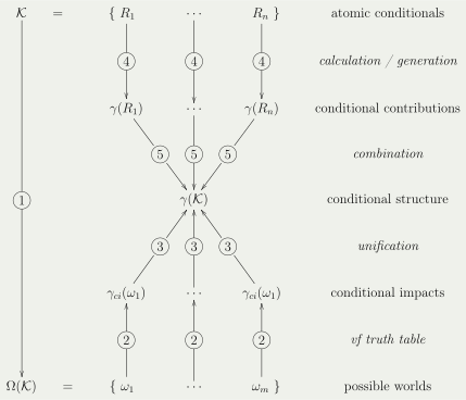
Figure 4.1 Conditional Structure, Conditional Contribution and Conditional Impact

Figure 4.1 gives an overview of the relationship of CSs and atomic conditionals which we will investigate in the upcoming chapters. The figure shows also the the traditional way of CS generation as shown in section 2.3. We describe the steps shown in the figure in order to make it more transparent why the concepts of the current chapter are introduced.

A given atomic knowledge base $\kb$ consists of atomic conditionals $\R_1,\cdots,\R_n$ . Steps 1 to 3 show how the CS $\gamma(\kb)$ can be constructed by the methods introduced in chapter 2. In step 1 the set of possible worlds $\Omega(\kb)$ is derived from the ground atoms of $\kb$ . In step 2 the conditional impacts $\gci(\omega_1),\cdots,\gci(\omega_m)$ of these possible worlds are read from the lines of the vf truth table of $\kb$ . Finally, in step 3 all conditional impacts are unified to the CS $\gamma(\kb)$ . This method requires to look through the complete vf truth table of $\kb$ .

Whilst the conditional impacts are derived from the possible worlds, the conditional contributions are derived from the conditionals.

Steps 4 and 5 symbolize alternative ways for the construction of $\gamma(\kb)$ , which are investigated in this thesis. In step 4 we first either calculate or generate the CS of each single atomic conditional of $\kb$ , i.e. all conditional contributions of $\kb$ , which then in step 5 get combined to the CS $\gamma(\kb)$ . In chapter 6 we will investigate ways to calculate and in chapter 7 ways to generate conditional contributions. In chapter 9 we will show, how these CSs can be combined, so that they form the CS of an atomic knowledge base.

We want to emphasize again that all CSs in this and the following chapters have been constructed by the common method $\gamma_{tab}$ as defined in section 2.3, mostly by making use of the KReator tool as introduced in section 2.4. So even if we show alternative ways of CS construction we still checked all results by applying the common method.

4.1 Atomic Conditionals

This section introduces atomic conditionals, which will be used throughout this thesis.

We start with a definition of all sub-types of atomic conditionals.

Definition 17 (Types of Conditionals)

A c-conditional is a FOPCL conditional of the form $\big<\big(~C(V_1,\cdots,V_n)~|~\top~\big),~\xi~\big>$ , i.e. an op-probabilistic conditional which has exactly one predicate symbol in the conclusion and no predicate symbol in the antecedence.

A ca-conditional is a FOPCL conditional of the form $\big<\big(~C(V_1,\cdots,V_n)~|~A(W_1,\cdots,W_m)~\big),~\xi~\big>$ with $C\neq A$ , i.e. an op-conditional which has exactly one predicate symbol in the conclusion and exactly one predicate symbol in the antecedence and the two predicate symbols are different.

A cc-conditional is a FOPCL conditional of the form $\big<\big(~C(V_1,\cdots,V_n)~|~C(W_1,\cdots,W_n)\big),~\xi~\big>$ , i.e. an op-conditional which has exactly one predicate symbol in the conclusion and the same predicate symbol as the only predicate symbol in the antecedence.

A cac-conditional is either a ca-conditional or a cc-conditional.

Note that the definition of the cac-condtional does not include c-conditionals.

Definition 18 (Atomic Conditional, Knowledge Base)

An atomic conditional is either a c-conditional or a ca-conditional or a cc-conditional.

The set of all atomic conditionals is denoted by $\aR$ .

For an atomic conditional $R$ , the predicate symbol in the conclusion is denoted by $C$ and predicate symbol in the antecedence is denoted by $A$ .

It is $\kba \subseteq \aR$ an atomic knowledge base.

The following proposition shows that for atomic conditionals only a single criteria for the determination of imbalanced usage of ground atoms is required.

Proposition 3 (Imbalanced Use within an Atomic Knowledge Base)

For an atomic knowledge base $\kba$ , the case of imbalanced use of combinations of ground atoms is covered by the case of imbalanced use of ground atoms.

Proof

It follows from definition 5 that both types of imbalanced use occur locally within a conditional $\Ra\in\kba$ , i.e. any imbalanced use held by $\Ra$ is not caused by nor does it affect any other conditional $\R^{a'}\in\kba$ . It is therefore sufficient to show that the case of imbalanced use of combinations of ground atoms within $\Ra$ is covered by the case of imbalanced use of ground atoms within $\Ra$ .

Furthermore it follows from definition 5 that in order for an imbalanced use to occur, at least two predicate symbols ( $P$ and $P'$ ) must be identical within $\Ra$ , so that $|p|_{\gnd(\Ra)} < |p'|_{\gnd(\Ra)}$ . For the case of imbalanced use of combinations of ground atoms by $\Ra$ at least two times two predicate symbols ( $P$ and $P'$ as well as $Q$ and $Q'$ ) must be identical within $\Ra$ , so that $\Ra$ would need to include at least four predicate symbols.

An atomic conditional consists of a maximum of two predicate symbols - one for the conclusion ( $C$ ), one for the antecedence ( $A$ ). This means that for an atomic conditional an imbalanced use can only occur if $C = A$ .□

4.2 Negation

This thesis does not explicitly treat cases in which one more more of the predicates within an atomic conditional are negated. Although we assume that negation will not substantially change the upcoming results, we currently cannot proof this.

4.3 Conditional Contribution

In this section we define the conditional contribution, which is the CS of a single atomic conditional. In the upcoming chapters we will mainly investigate ways to calculate or generate such conditional contributions. In chapter 9 we will show a way to combine the different conditional contributions of the conditionals of an atomic knowledge base to the related CS.

Definition 19 (Conditional Contribution)

Let $\R \in \kb$ be an atomic conditional.

The conditional contribution (CC) of conditional $R$ is

\gamma(\R) := \bigcup_{\omega\in\Omega(\kb)} vf_R(\omega)

the set of vf-pairs generated by conditional $\R$ .

Example 13 (Conditional Contribution)

Continuing from example 9 and example 7.

The conditional contribution of the atomic conditionals in $\kb$ and $\kb'$ can be read from the vf truth table of example 7.

$\gamma(\R_1)$	$=$	$\{$	$(0,0),$	$(0,1),$	$(1,0),$	$(0,2),$	$(2,0)$	$\}$
$\gamma(\R_2)$	$=$	$\{$	$(0,2),$	$(1,1),$	$(2,0)$	$\}$
$\gamma(\R_{2-1})$	$=$	$\{$	$(0,1),$	$(1,0)$	$\}$
$\gamma(\R_{2-2})$	$=$	$\{$	$(0,1),$	$(1,0)$	$\}$

4.4 Common Appearance

A FOPCL knowledge base usually includes many different conditionals. As we have seen in definition 11, the conditional impact of a specific possible world $\omega$ includes one vf-pair per conditional. The unification of all conditional impacts of a knowledge base then forms the CS, as defined by definition 13.

In this section we introduce the common appearance tables, which visualize which vf-pairs of the conditional contributions of two conditionals appear commonly within a conditional impact of a knowledge base, as expressed in the following definition.

Definition 20 (Common Appearance)

Let $\kb$ be an FOPCL knowledge base and let and $\omega\in\Omega(\kb)$ be a possible world of $\kb$ . Let $\gamma(\omega)$ be the conditional impact of $\omega$ and let $\vf_1, \vf_2 \in \gamma(\omega)$ be two vf-pairs within the conditional impact of $\omega$ .

Then $\vf_1$ and $\vf_2$ have a common appearance CA.

Example 14 (Common Appearance)

Continuing from example 9.

Within $\gamma(\omega_1)$ the vf-pair $(0,~1)$ shares a common appearance with $((0,~2)$ , as $(0,~1),~(0,~2)\in\gamma(\omega_1) = (~(0,~1),~(0,~2)~)$ .

From chapter 9 on common appearances will be used e.g. for finding specific patterns between conditional contributions which hint towards certain characteristics of the related knowledge base, e.g. the two conditionals could hold a balanced sharing. In order to better visualize these patterns we now introduce the common appearance table.

Definition 21 (Common Appearance Table)

Let $R_1, R_2 \in \kb$ .

Then the common appearance table (CA-table) of $\R_1$ and $\R_2$ is a table which shows

the vf-pairs of $\R_1$ vertically as line headings; and
the vf-pairs of $\R_2$ horizontally as column headings; and
in each cell of the table, if the related vf-pairs have a common appearance, a " $*$ " indicator.

The set of common appearances of $\R_1$ and $\R_2$ is denoted by $CA(\R_1,\R_2)$ .

As the CA-table reflects the complete set set of common appearances we also use $CA(\R_1,\R_2)$ as an indicator for the CA-table of $\R_1$ and $\R_2$ .

Example 15 (Common Appearance Table)

Continuing from example 14.

Table 4.1 shows $CA(\R_1,\R_2)$ , i.e. the CA-table for $\R_1$ and $\R_2$ .

Table 4.1
$CA(\R_1,\R_2)$	$(0,~2)$	$(1,~1)$	$(2,~0)$
$(0,~0)$	$*$	$*$	$*$
$(0,~1)$	$*$	$*$
$(1,~0)$		$*$	$*$
$(0,~2)$	$*$	$*$
$(2,~0)$		$*$	$*$

Table 4.1: CA-table of

R_1

and

R_2

of Example 15

4.5 $\vf$ -Pair Operations

In this section we define addition and scalar multiplication for vf-pairs.

Definition 22 (vf-Pair Addition)

The operation $+ : \VF\times\VF \rightarrow \VF$ with $((a,~b),~(a',~b')) \mapsto (a+a',~b+b')$ for all $((a,~b),~(a',~b'))\in\VF\times\VF$ is called the vf-pair addition or simply vf addition.

The neutral element of the vf addition is the vf-pair $(0,~0)$ .

No inverse element is defined, as we don’t assume negative values for vf-pairs.

Example 16 (vf-Pair Addition)

Let $\vf_1 = (2,~0)$ and $\vf_2 = (1,~1)$ be two vf-pairs.

It is $\vf_1 + \vf_2 ~=~ (2,~0) + (1,~1)~=~(2+1,~0+1)~=~(3,~1)$ .

From definition 22 it is trivial to see that the vf-pair addition is associative and commutative. We nevertheless proof the following proposition, but will not further proof similar statements.

Proposition 4 (vf-Pair Addition is Associative and Commutative)

The vf-pair addition is associative and commutative.

Proof

Let $(a,~b),~(c,~d),~(e,~f)$ be vf-pairs.

It is $(a,~b) + ((c,~d)+(e,~f)) = (a,~b) + (c+e,~d+f) = (a+c+e,~b+d+f) = (a+c,~b+d) + (e,~f) = ((a,~b)+(c,~d))+(e,~f)$ and therefore the vf-pair addition is associative.

It is $(a,~b) + (c,~d) = (a+c,~b+d) = (c+a,~d+b) = (c,~d) + (a,~b)$ and therefore the vf-pair addition is commutative.□

Definition 23 (vf-Pair Scalar Multiplication)

The operation $\cdot : \mathbb{N}\times\VF$ with $(r,~(a,~b)) \mapsto (r\cdot a,~r\cdot b)$ for all $(r,~(a,~b))\in\mathbb{N}\times\VF$ is called vf skalar multiplication or simply scalar multiplication.

Example 17 (vf-Pair Scalar Multiplication)

Let $vf = (2,3)$ be a vf-pair.

It is $5\cdot \vf ~=~ 5\cdot(2,~3) ~=~(5\cdot 2,~5\cdot 3)~=~(10,~15)$ .

It is trivial to see that the scalar multiplication for vf-pairs is associative.

4.6 Maximum Ordered Sums

In this section we introduce the concept of maximum ordered sums, which will first of all allow us to shorten the notation of CSs. Furthermore they will also simplify certain calculation and generation steps, which will be shown in later chapters. They also play an important role when it comes to the transformation of certain types of CSs as discussed in chapter 11.

Definition 24 (Maximum Ordered Sums)

Let $n,i,j \in \mathbb{N}_0$ be positive integers.

The (set of) maximum ordered sums (MOS) of $n$ is the $n+1$ -tuple

[n] := (~(i,~j)~|~ 0 \leq i,j \leq n,~i+j = n~),

whereby the tuple is sorted first by $i$ and then by $j$ .

A partial MOS is a subset of a MOS.

Note that we did not define a notation for a partial MOS. Partial MOSs will always be written as the list of the individual ordered sums they contain.

Example 18 (Maximum Ordered Sums)

The MOS of $3$ is $[3] = (~(0,3),~(1,2),~(2,1)~,(3,0)~)$ .

It is $(~(0,6),~(2,4),~(4,2)~,(6,0)~)$ a partial MOS, as it is a subset of $[6]$ .

Proposition 5 (Size of MOS)

Let $n\in\IN_0$ be a non-negative integer.

Then it holds that $|[n]| = n+1$ .

Proof

For every $n \in \mathbb{N}$ there exist exactly $n+1$ numbers $i$ between $0$ and $n$ .

For each such $i$ there exists exactly one $j$ for which $i+j=n$ , as it holds for all $j'\in\mathbb{N}$ that if $j'>j$ then $i+j' > i+j = n$ and if $j'<j$ then $i+j' < i+j = n$ .

It follows that for every $i$ there is exactly one tuple $(i,j)$ in $[n]$ , so that

[n] = (~(0,~n),~(1,~n-1),~\cdots,~(n-1,~1),~(n,~0)~).

It follows that $|[n]| = n+1$ .□

Definition 25 (Multiples of a MOS (Scalar Multiplication))

Let $n \in \mathbb{N}_0$ be a positive integer.

The $k$ ’th mulitple of $[n]$ is the partial MOS

k[n] := (~(k \cdot i,~k \cdot j)~|~(i,~j) \in [n] ).

We write $k(i,~j)$ instead of $(k\cdot i,~k \cdot j)$ .

Example 19 (Multiples of a MOS (Scalar Multiplication))

It holds that $2[3] = \big(~2(0,3),~2(1,2),~2(2,1),~2(3,0)~) = (~(0,6),~(2,4),~(4,2),~(6,0)~\big)$ and $3[2] = \big(~3(0,2),~3(1,1),~3(2,0)~) = (~(0,6),~(3,3),~(6,0)~\big)$ , so that $2[3] \neq 3[2]$ .

The MOS and the related scalar multiplication first of all allow us a shorter notation of conditional contributions, wherever possible.

Example 20 (Conditional Contributions and MOS)

Continuing from example 13.

We can express the CSs also by means of MOS.

$\gamma(R_1)$	$=$	$\{~[0],~[1],~2[1]~\}$
$\gamma(R_2)$	$=$	$\{~[2]~\}$
$\gamma(R_{2-1})$	$=$	$\{~[1]~\}$
$\gamma(R_{2-2})$	$=$	$\{~[1]~\}$

Note that not all conditional contributions of atomic conditionals necessarily create a complete MOS but sometimes only a partial MOS.

Unfortunately an addition of MOS’ cannot be easily defined in a way that it would make sense for the purpose of conditional contributions and CSs. This will be further investigated in section 6.5.

4.7 Possible World Segments

In this chapter we will split the possible worlds of a conditional into two parts or segments. The first segment will be based on all admissible ground atoms of the conclusion predicate of the conditional, the other segment will be based on the ground atoms of the antecedence predicate of the conditional. These two segments can overlap with respect to their ground atoms. We will also introduce a combination function which allows to re-combine possible world segments.

In later parts of this thesis, mainly in chapter 7 we will create segments of segments to allow for a faster generation of the conditional contribution. In order to allow for such flexibility, we start off with a very general definition of the possible world segments.

Definition 26 (Possible World Segments)

Let $X$ and $Y$ be two sets of ground atoms with $X\subseteq Y$ .

Then $\Omega(X)$ is a set of possible world segments of $\Omega(Y)$ . A possible world $\omega^x\in\Omega(X)$ is called a possible world segment or, in short, segment.

We write $\Omega(X) \subseteq \Omega(Y)$ to indicate that $\Omega(X)$ is a possible world segment of $\Omega(Y)$ .

Let $\Rcac = \big<\big(~C~|~A~\big),~\xi~\big>$ be a cac-conditional.

The c-atoms of $\Rcac$ are the ground atoms which occur in the conclusion of an admissible ground instance of $\Rcac$ and are denoted by $\cat(\Rcac)$ , i.e. $\cat(\Rcac) = \{~c~|~\big<(c|a)\big>\in\gnd(\Rcac)~\}$ .

The a-atoms of $\Rcac$ are the ground atoms which occur in the antecedence of an admissible ground instance of $\Rcac$ and are denoted by $\aat(\Rcac)$ , i.e. $\aat(\Rcac) = \{~a~|~\big<(c|a)\big>\in\gnd(\Rcac)~\}$ .

The set of c-segments of $\Rcac$ is $\OmegaC(\Rcac) = \Omega(\cat(\Rcac))$ . A possible world $\omega^c\in\OmegaC(\Rcac)$ is called a c-segment.

The set of a-segments of $\Rcac$ is $\OmegaA(\Rcac) = \Omega(\aat(\Rcac))$ . A possible world $\omega^a\in\OmegaC(\Rcac)$ is called an a-segment.

The next definition allows for easier notation of possible world segments.

Definition 27 (Index of Ground Atoms in Possible World Segments)

Let $\Rcac$ be a cac-conditional.

Let $i\in\IN$ be an unique index assigned to every $c\in\cat(\Rcac)$ , with $1\leq i\leq|\cat(\Rcac)|$ and let $j\in\IN$ be an unique index assigned to every $a\in\aat(\Rcac)$ , with $1\leq j\leq|\aat(\Rcac)|$ .

Let $\omega^c\in\Omega^C(\Rcac)$ and $\omega^a\in\Omega^A(\Rcac)$ .

We denote $\omega^c$ also as $\omega^c_{(i_1,\cdots,i_l)}$ , whereby $i_1,\cdots,i_l$ are the indexes of c-atoms which are verified by $\omega^c$ . We write $\omega^c_{()}$ if no c-atom is verified by $\omega^c$ .

We denote $\omega^a$ also as $\omega^a_{(j_1,\cdots,j_k)}$ , whereby $j_1,\cdots,j_l$ are the indexes of a-atoms which are verified by $\omega^a$ . We write $\omega^a_{()}$ if no a-atom is verified by $\omega^a$ .

In the case that two segments have overlapping ground atoms, the indexes assigned to those ground atoms are identical in both segments.

Example 21 (Possible World Segments)

Let $s = \{~a,~b,~c~\}$ be a sort, $V,W$ be variables over sort $s$ and ${\Rcac = \big<~\big(~C(V)~|~A(W)~\big),~V\neq c~\big>}$ .

Then we get $\cat(\Rcac) = \{~C(a),~C(b)~\}$ and $\aat(\Rcac) = \{~A(a),~A(b),~A(c)~\}$ . $\OmegaC(\Rcac)$ is the set of c-segments which assigns all possible combinations of truth values to all c-atoms of $\Rcac$ . Table 4.2 shows the c-segments of $\Rcac$ .

Table 4.2
$\omega^c_{i}\in\OmegaC(\Rcac)$	$C(a)$	$C(b)$
$i:$	$2$	$1$
$\omega^c_{()}$	$0$	$0$
$\omega^c_{(1)}$	$0$	$1$
$\omega^c_{(2)}$	$1$	$0$
$\omega^c_{(1,2)}$	$1$	$1$

Table 4.2: C-Segments of

R^{cac}

of Example 21

$\OmegaA(\Rcac)$ is the set of a-segments which assign all possible combinations of truth values to all a-atoms of $\Rcac$ . Table 4.3 shows the a-segments of $\Rcac$ .

Table 4.3
$\omega^a_{i}\in\OmegaA(\Rcac)$	$A(a)$	$A(b)$	$A(c)$
$j:$	$3$	$2$	$1$
$\omega^a_{()}$	$0$	$0$	$0$
$\omega^a_{(1)}$	$0$	$0$	$1$
$\omega^a_{(2)}$	$0$	$1$	$0$
$\omega^a_{(1,2)}$	$0$	$1$	$1$
$\omega^a_{(3)}$	$1$	$0$	$0$
$\omega^a_{(1,3)}$	$1$	$0$	$1$
$\omega^a_{(1,2)}$	$1$	$1$	$0$
$\omega^a_{(1,2,3)}$	$1$	$1$	$1$

Table 4.3: A-Segments of

R^{cac}

of Example 21

The next definition allows us to differentiate between those segments which only entail a single ground atom and those which entail several ground atoms.

Definition 28 (Canonical and Composed Segments)

Let $\Rcac$ be a cac-conditional.

An a-segment $\omega^a\in\OmegaA(\Rcac)$ is called a canonical a-segment iff exactly one a-atom is verified by $\omega^a$ .

An a-segment $\omega^a\in\OmegaA(\Rcac)$ is called a composed a-segment iff more than one a-atom is verified by $\omega^c$ .

A c-segment $\omega^c\in\OmegaC(\Rcac)$ is called a canonical c-segment iff exactly one c-atom is verified by $\omega^c$ .

Note that we did not define a specific name for the a-segment $\omega^a_{()}$ which does not verify any a-atom. It can be regarded as a canonical a-segment but for the purpose of this thesis this makes no difference.

Example 22 (Canonical and Composed Segments)

Continuing from example 21

The canonical c-segments of $\Rcac$ are $\omega^c_{(1)}$ and $\omega^a_{(2)}$ , as in each of them only one c-atom is verified.

The canonical a-segments of $\Rcac$ are $\omega^a_{(1)},~\omega^a_{(2)}$ and $\omega^a_{(3)}$ , as in each of them only one a-atom is verified.

The composed a-segments of $\Rcac$ are $\omega^a_{1,2}$ , $\omega^a_{1,3}$ , $\omega^a_{2,3}$ and $\omega^a_{1,2,3}$ .

The naming of the different a-segments already gives a hint on how they will be used later, i.e. we will show in the upcoming chapters that for ca-conditionals the vf-pairs "counted" or "contributed" by composed a-segments are the sums of the vf-pairs of canonical a-segments.

The following definition names the different relations that the sets of entailed ground atoms of an c- and an a-segment can have.

Definition 29 (Dependency Between C- and A-Segments)

Let $\Rcac$ be a cac-conditional.

We say that the possible world segments of $\Rcac$ are

independent iff $\cat(\Rcac) \cap \aat(\Rcac) = \emptyset$ ;
identical iff $\cat(\Rcac) = \aat(\Rcac)$ ; and
overlapping iff $\cat(\Rcac) \neq \aat(\Rcac) ~ \wedge ~ \cat(\Rcac) \cap \aat(\Rcac) \neq \emptyset$ .

If the possible world segments of $\Rcac$ are overlapping, then the overlap of $\Rcac$ is defined as $\ovl(\Rcac) = \cat(\Rcac)\cap\aat(\Rcac)$ and the difference of $\Rcac$ is defined as $\diff(\Rcac) = \herbrand(\Rcac)\backslash\ovl(\Rcac)$

Example 23 (Dependency Between C- and A-Segments)

Let $C$ and $A$ be unary predicate symbols, which variables all range over sort $s= \{~a,~b,~c~\}$ .

Let $\Rcac_1 = \big<\big(~C(V)~|~A(W)~\big), ~V\neq c,~W\neq a~\big>$ . It is $\cat(\Rcac_1) = \{~C(a),~C(b)~\}$ and $\aat(\Ra_1) = \{~A(b),~A(c)~\}$ and therefore the possible world segments of $\Rcac_1$ are independent, as $\cat(\Rcac_1) \cap \aat(\Rcac_1) = \emptyset$ , so that ${\ovl(\Rcac_1)=\emptyset}$ and ${\diff(\Rcac_1)=\{~C(a),~C(b),~A(b),~A(c)~\}}$ .

Let $\Rcac_2 = \big<\big(~C(V)~|~C(W)~\big), ~V\neq c,~W\neq a~\big>$ . It is $\cat(\Rcac_2) = \{~C(a),~C(b)~\}$ and $\aat(\Rcac_2) = \{~C(b),~C(c)~\}$ and therefore the possible world segments of $\Rcac_2$ are overlapping, as $\cat(\Rcac_2) \neq \aat(\Rcac_2) ~ \wedge ~ \cat(\Rcac_2) \cap \aat(\Rcac_2) \neq \emptyset$ . Then we have $\ovl(\Rcac_2) = \{~C(b)~\}$ and $\diff(\Rcac_2) = \{~C(a),~C(c)~\}$ .

Let $\Rcac_3 = \big<\big(~C(V)~|~C(W), W\neq c~\big), ~V\neq c,~W\neq c~\big>$ . Then we have $\cat(\Rcac_3) = \{~C(a),~C(b)~\} = \aat(\Rcac_3)$ and therefore the possible world segments of $\Rcac_3$ are identical.

Now that we split the possible worlds into segments we also want to be able to combine segments together. As long as there are no overlapping ground atoms in the segments this is no problem. But if there is an overlap we have to define how to handle it. We will therefore define the combination of possible worlds in such a way that the same truth value has to be assigned to overlapping ground atoms in order to combine the related segments. Else the two segments cannot be combined.

Definition 30 (Semantical Combination of Possible Worlds)

Let $GA_1$ and $GA_2$ be two sets of ground atoms.

Let $\omega_1\in\Omega(GA_1)$ and $\omega_2\in\Omega(GA_2)$ be two possible worlds, consisting of specific truth values assigned to the sets of ground atoms $GA_1$ and $GA_2$ .

We call $\omega\in\Omega(GA_1 \cup GA_2)$ the semantical combination of $\omega_1$ and $\omega_2$ iff $\omega$ assigns the same truth values as $\omega_1$ and $\omega_2$ to those ground atoms which appear both in $GA_1$ and $GA_2$ .

Note that in the above definition the two sets of ground atoms are not mandated to be mutually exclusive, i.e. there might be an overlap between them. The unification will only work if the truth values assigned to identical ground atoms within the overlap is identical. This will be shown in more detail in example 26.

Example 24 (Semantical Combination of Possible Worlds)

Continuing from example 21

We look at the two possible worlds $\omega_{18},\omega_{21}\in\Omega(\Rcac)$ , which are shown in table 4.4.

Table 4.4
$\omega_{i}\in\Omega(\Rcac)$	$C(a)$	$C(b)$	$A(a)$	$A(b)$	$A(c)$
$\vdots$
$\omega_{18}$	$1$	$0$	$0$	$1$	$0$
$\vdots$
$\omega_{21}$	$1$	$0$	$1$	$0$	$1$
$\vdots$

Table 4.4: Two C-Segments of Example 24

It is $\omega_{18}$ the semantical combination of $\omega^c_{(2)}$ and $\omega^a_{(2)}$

It is $\omega_{21}$ the semantical combination of $\omega^c_{(2)}$ and $\omega^a_{(1,3)}$

Note that the c-segment $\omega^c_{(2)}$ is a possible world segment of $\omega_{18}$ as well as of $\omega_{21}$ , as in all of them the ground atoms $C(a)$ and $C(b)$ are set to the same truth values. Obviously, there are more possible worlds $\omega\in\Omega(\Rcac)$ for which the ground atoms are set in the same way as in $\omega^c_{(2)}$ than shown here.

Definition 31 (Semantical Combination Function)

The binary operator $\timesM$ is the semantical combination function which creates the semantical combination of two possible worlds.

We also use $\timesM$ to create all possible semantical combinations of all possible worlds within two sets of possible worlds.

Example 25 (Semantical Combination Function)

Continuing from example 24.

It is $\omega_{18} = \omega^c_{(2)} \timesM \omega^a_{(2)}$ and $\omega_{21} = \omega^c_{(2)} \timesM \omega^a_{(1,3)}$

Example 26 (Semantical Combination Function for Sets of Possible Worlds)

Continuing from example 23.

Table 4.5 shows $\OmegaC(\Rcac_1) \timesM \OmegaA(\Rcac_1)$ , i.e. the possible worlds which are generated by the semantical combination of the c-segments and the a-segments of $\Rcac_1$ .

Table 4.5
		$\scriptsize{\OmegaA(\Rcac_1)}$
		$00$	$01$	$10$	$11$
$\OmegaC(\Rcac_1)$	$00$	$0000$	$0001$	$0010$	$0011$
	$01$	$0100$	$0101$	$0110$	$0111$
	$10$	$1000$	$1001$	$1010$	$1011$
	$11$	$1100$	$1101$	$1110$	$1111$

Table 4.5: Unification of

\Omega ^C(R^{cac}_1)

and

\Omega ^A(R^{cac}_1)

of Example 26

Table 4.6 shows $\OmegaC(\Rcac_2) \timesM \OmegaA(\Rcac_2)$ , whereby the truth values of the c-/a-atoms which are overlapping in the c-/a-segments are indicated in brackets.

Table 4.6
		$\scriptsize{\OmegaA(\Rcac_2)}$
		$(0)0$	$(0)1$	$(1)0$	$(1)1$
$\OmegaC(\Rcac_2)$	$0(0)$	$000$	$001$	$-$	$-$
	$0(1)$	$-$	$-$	$010$	$011$
	$1(0)$	$100$	$101$	$-$	$-$
	$1(1)$	$-$	$-$	$110$	$111$

Table 4.6: Unification of

\Omega ^C(R^{cac}_2)

and

\Omega ^A(R^{cac}_2)

of Example 26

From example 25 we can see that the semantical combination function does not necessarily always combine all c-segments with all a-segments of a given conditional. As long as there is an overlap only the segments which assign the same value to the overlapping ground atoms will be combined.

4.8 Atomic Counting Functions

The atomic counting functions as defined by this section are an alternative definition of the counting functions defined in section 2.3. Both, the atomic as well as the traditional counting functions, result in the same values. But whilst the traditional counting functions operate on complete possible worlds, the atomic counting functions operate on possible world segments.

Definition 32 (Atomic Counting Functions)

Let $\Rcac \in \kba$ be an cac-conditional with $\Rcac = \big<~(~C~|~A~),~\xi~\big>$ .

Let $\omega^c$ be a c-segment and $\omega^a$ an a-segment of $\Rcac$ .

Then

$\vera_{\Rcac}(\omega^c,~\omega^a) := \big|\big\{~\big<(c|a)\big>~\in\gnd(\Rcac)~\big|~\omega^c \models c,~\omega^a \models a~\big\}\big|$ is the atomic counting function which counts the number of ground instances of conditional $\Rcac$ of which the related c-atoms are verified by c-segment $\omega^c$ and the related a-atoms are verified by a-segment $\omega^a$ ;
$\fala_{\Rcac}(\omega^c,~\omega^a) := \big|\big\{~\big<(c|a)\big>~\in\gnd(\Rcac)~\big|~\omega^c \models \neg c,~\omega^a \models a~\big\}\big|$ is the atomic counting function which counts the number of ground instances of conditional $\Rcac$ of which the related c-atoms are falsified by c-segment $\omega^c$ and the related a-atoms are verified by a-segment $\omega^a$ ;
$\vfa_{\Rcac}(\omega^c,~\omega^a) := (~\vera_{\Rcac}(\omega^c,~\omega^a),~\fala_{\Rcac}(\omega^c,~\omega^a)~)$ is an atomic vf-pair, i.e. the tuple consisting of the values of the atomic counting functions.

The following proposition states that the traditional and the atomic counting functions result in the same values.

Proposition 6 (Equality of Counting Function Definitions)

Let $\Rcac_i \in \kb$ be an cac-conditional and $\omega_j \in \Omega(\Rcac)$ be a possible world. Let $\omega^c$ be the c-segment of $\omega_j$ and let $\omega^a$ be the a-segment of $\omega_j$ , so that $\omega^c\timesM\omega^a = \omega_j$ .

It is $\vf_{i,j} = \vf_{\Rcac_i}(\omega_j) = \vfa_{\Rcac_i}(\omega^c,~\omega^a)$ .

Proof

Due to definition 10 it is $\ver_{i,j} = \{~\big<\big(c|a\big)\big>~\in\gnd(\Rcac_i)~|~\omega_j\models c \wedge a~\}$ , whereby $c$ is any ground atom of $\Rcac_i$ which appears in the conclusion part of any admissible grounding of $\Rcac_i$ . As $c$ is used as a ground atom in $\omega_j$ and as no further conditions are given, it holds that $\omega_j \models c$ iff the ground atom $c$ is verified by $\omega_j$ . Therefore the entailment of $c$ by $\omega_j$ depends only on the setting of the ground atom $c$ within $\omega_j$ .

As $\omega^c \in \OmegaC(\Rcac_i)$ it holds that $\omega^c$ covers all ground atoms $\cat(\Rcac_i) = \{~c~|~\big<\big(c|a\big)\big>\in\gnd(\Rcac_i)~\}$ , i.e. $\omega^c$ assigns truth values to every ground atom which occurs in the conclusion part of any admissible grounding of $\Rcac_i$ .

If the ground atom $c$ occurs not only in the conclusion part of $\Rcac_i$ , but also in its antecedence part, then it holds due to condition $\omega^c \timesM \omega^a = \omega_j$ that $(\omega^c \models c) \equiv (\omega^a \models c)$ . and $(\omega^c \models c) \equiv (\omega_j \models c)$ .

In the same way it can be shown that $\omega_j \models a ~\equiv~\omega^a \models a$ .

Therefore it holds that

$\ver_{i,j}$	$= \big\|\big\{~\big<\big(c\|a\big)\big>~\in\gnd(\Rcac_i)~\big\|~\omega_j\models c \wedge a~\big\}\big\|$
	$= \big\|\big\{~\big<\big(c\|a\big)\big>~\in\gnd(\Rcac_i)~\big\|~\omega_j\models c,~\omega_j \models a~\big\}\big\|$
	$= \big\|\big\{~\big<\big(c\|a\big)\big>~\in\gnd(\Rcac_i)~\big\|~\omega^c\models c,~\omega^a \models a~\big\}\big\|$
	$= \vera_{\Rcac_i}(\omega^c,\omega^a)$

In the same way it can be shown that it holds that $\fal_{i,j} = \fala_{\Rcac_i}(\omega^c, \omega^a)$ .

It follows that

$\vf_{i,j}$	$= (\ver_{i,j}, \fal_{i,j})$
	$= (\vera_{\Rcac_i}(\omega^c,\omega^a), \fala_{\Rcac_i}(\omega^c,\omega^a))$
	$= \vfa_{\Rcac_i}(\omega^c,\omega^a).$

□

The above definition 32 and proposition 6 do not work for c-conditionals, i.e. for conditionals which don’t have any antecedence predicate. For c-conditionals we will further use the traditional counting functions of definition 10. We will see in section 6.1 how the atomic counting functions nevertheless can be applied to c-conditionals.

For proposition 6 it is important to note that due to the condition $\omega^c\timesM\omega^a = \omega_j$ it holds that if $\cat(\Rcac_i)\cap\aat(\Rcac_i)\neq\emptyset$ , i.e. if one or more ground atoms are used as both, c-atoms and a-atoms, then only those $\omega^c$ and $\omega^a$ can appear in the related atomic counting functions which assign the same truth values to the related ground atoms. This guarantees that the counting functions operate only on those segments which are both part of a possible world $\omega_j\in\Omega(\Rcac_i)$ .

The following example shows how the atomic counting functions work in different cases, i.e. if the possible world segments are independent, overlapping or identical.

Example 27 (Equality of Counting Function Definitions)

Continuing from example 23.

For $\Rcac_1 = \big<\big(~C(V)~|~A(W)~\big), ~V\neq c,~W\neq a~\big>$ , let $\omega_9 \in \Omega(\Rcac_1)$ with $\omega_9 = \omega^c_{(2)}\timesM\omega^a_{1}$ whereby $\omega^c_{(2)}\in\OmegaC(\Rcac_1)$ and $\omega^a_{(1)}\in\OmegaA(\Rcac_1)$ as shown in table 4.7. In this case the possible world segments are independent.

Table 4.7
	$\omega^c$		$\omega^a$
	$C(a)$	$C(b)$	$A(b)$	$A(c)$	$\vf$
	$\omega^c_{(2)}$	$\omega^c_{(1)}$	$\omega^a_{(2)}$	$\omega^a_{(1)}$
$\vdots$
$\omega_9$	$1$	$0$	$0$	$1$	$(1,~1)$
$\vdots$

Table 4.7: Extract from vf Truth Table of

R^{cac}_1

(independent segments) of Example 27

It is $\ver_{\Rcac_1}(\omega_9) = (1,~1)$ as

$\omega_9 \models A(c) \wedge \omega_9\models C(a)$ and
$\omega_9 \models A(c) \wedge \omega_9\models \neg C(b)$ and
$\omega_9 \not\models A(b)$ .

It is $\vera_{\Rcac_1}(\omega^c_{(2)},\omega^a_{(1)}) = (1,~1)$ as

$\omega^a_{(1)} \models A(c) \wedge \omega^c_{(2)}\models C(a)$ and
$\omega^a_{(1)} \models A(c) \wedge \omega^c_{(2)}\models \neg C(b)$ and
$\omega^a_{(1)} \not\models A(b)$ .

For $\Rcac_2 = \big<\big(~C(V)~|~C(W)~\big), ~V\neq c,~W\neq a~\big>$ let $\omega_3=\omega^c_{(1)}\timesM\omega^a_{(1,2)}$ whereby $\omega^c_{(1)}\in\OmegaC(\Rcac_2)$ and $\omega^a_{(1,2)}\in\OmegaA(\Rcac_2)$ , as shown in table 4.8. In this case the possible world segments are overlapping with $\ovl(\Rcac_2) = \{~C(b)~\}$ .

Table 4.8
		$\omega^a$
		$\overbrace{~~~~~~~~~~~~~~}$
	$\omega^c$
	$\overbrace{~~~~~~~~~~~~~~}$
	$C(a)$	$C(b)$	$C(c)$	$\vf$
	$\omega^c_{(2)}$	$\omega^c_{(1)}$
		$\omega^a_{(1)}$	$\omega^a_{(2)}$

$\vdots$
$\omega_3$	$0$	$1$	$1$	$(2,~2)$
$\vdots$

Table 4.8: Extract from vf Truth Table of

R^{cac}_2

of Example 27

It is $\ver_{\Rcac_2}(\omega_3) = (2,~2)$ as

$\omega_3 \models C(c) \wedge \omega_3\models C(b)$ and
$\omega_3 \models C(b) \wedge \omega_3\models C(b)$ and
$\omega_3 \models C(c) \wedge \omega_3\models \neg C(a)$ and
$\omega_3 \models C(b) \wedge \omega_3\models \neg C(a)$ .

It is $\vera_{\Rcac_2}(\omega^c_{(1)},\omega^a_{(1,2)}) = (2,~2)$ as

$\omega^a_{(1,2)} \models C(c) \wedge \omega^c_{(1)}\models C(b)$ and
$\omega^a_{(1,2)} \models C(b) \wedge \omega^c_{(1)}\models C(b)$ and
$\omega^a_{(1,2)} \models C(c) \wedge \omega^c_{(1)}\models \neg C(a)$ and
$\omega^a_{(1,2)} \models C(b) \wedge \omega^c_{(1)}\models \neg C(a)$ .

For $\Rcac_3 = \big<\big(~C(V)~|~C(W), W\neq c~\big), ~V\neq c,~W\neq c~\big>$ let $\omega_2=\omega^c_{(2)}\timesM\omega^a_{(2)}$ whereby $\omega^c_{(2)}\in\OmegaC(\Rcac_3)$ and $\omega^a_{(2)}\in\OmegaA(\Rcac_3)$ as shown in table 4.9. In this case the possible world segments are identical.

Table 4.9
	$\omega^a = \omega^c$
	$C(a)$	$C(b)$	$\vf$
	$\omega^c_{(2)}$	$\omega^c_{(1)}$
	$\omega^a_{(2)}$	$\omega^a_{(1)}$
$\vdots$
$\omega_2$	$1$	$0$	$(1,~1)$
$\vdots$

Table 4.9: Extract from vf Truth Table of

R^{cac}_3

of Example 27

It is $\ver_{\Rcac_3}(\omega_2) = (1,~1)$ as

$\omega_2 \models C(a) \wedge \omega_2\models C(a)$ and
$\omega_2 \models C(a) \wedge \omega_2\models \neg C(b)$ and
$\omega_2 \not \models C(b)$ .

It is $\vera_{\Rcac_3}(\omega^c_{(2)},\omega^a_{(2)}) = (1,~1)$ as

$\omega^a_{(2)} \models C(a) \wedge \omega^c_{(2)}\models C(a)$ and
$\omega^a_{(2)} \models C(a) \wedge \omega^c_{(2)}\models \neg C(b)$ and
$\omega^a_{(2)} \not\models C(b)$ .

The following definition allows us to avoid mentioning the counting functions whenever we talk about vf-pairs related to a-segments, i.e. it allows us to say that an a-segment or an a-atom counts a certain number of c-atoms.

Definition 33 (A-Segments Counting C-Atoms)

Let $\Rcac$ be a cac-conditional. Let $\omega^a\in\OmegaA(\Rcac)$ be a a-segment of $\Rcac$ and let $\omega^c\in\OmegaC(\Rcac)$ be a c-segment of $\Rcac$ .

Let $n = \vera_{\Rcac}(\omega^c,\omega^a + \fala_{\Rcac}(\omega^c,\omega^a)$ .

We say that $\omega^a$ counts $n$ c-atoms of $\omega^c$ .

Let $\omega^a_{(t)}\in\OmegaA(\Rcac)$ be a canonical a-segment of $\Rcac$ with $t$ being the index of ground atom $a_t$ , so that it holds that $\omega^a_{(t)}\models a_t$ .

Let $m = \vera_{\Rcac}(\omega^c,\omega^a_{(j)} + \fala_{\Rcac}(\omega^c,\omega^a_{(j)})$ .

We say that $a_t$ counts $m$ c-atoms of $\omega^c$ .

4.9 Types of Instantiation Restrictions

In this section we will distinguish mainly two types of instantiation restrictions, which we will call local and non-local. This is done as these different types of instantiation restrictions have different influences on the counting functions of an FOPCL knowledge base.

In the following chapters we will find several propositions to hold for conditionals which are free of non-local instantiation restrictions. If we would not distinguish between local and non-local instantiation restrictions then these propositions would only hold for conditionals which are free of any instantiation restrictions at all.

We start with some definitions that make it easier for us to talk about instantiation restrictions.

Definition 34 (Types of Instantiation Restrictions)

We will refer to the different types of instantiation restrictions by simply indicating them as of type $V=c$ , type $V\neq c$ , type $V=W$ and type $V\neq W$ respectively.

We call type $V=c$ and type $V\neq c$ constant type instantiation restrictions and type $V=W$ and type $V\neq W$ variable type instantiation restrictions.

We will also say that a conditional is free of a certain kind of instantiation restrictions, if no such type of instantiation restriction is used by the conditional.

Example 28 (Types of Instantiation Restrictions)

Let $R_1=\big<\big(C(U)~\big|~A(b)\big),~U\neq a~\big>$ . $R_1$ includes two constant instantiation restrictions, one being of type $V=c$ implicitly denoted by the constant $b$ in $A(b)$ , the other ( $U\neq a$ ) being of type $V\neq c$ . $R_1$ is free of any type of variable instantiation restriction.

Let $R_2=\big<\big(C(X,Y)~\big|~A(X,X,Z)\big),~X\neq Y~\big>$ . $R_2$ includes variable instantiation restrictions of the following types:

type $V=W$ within different predicates due to variable $X$ occurring in both the conclusion and the antecedence predicate;
type $V=W$ within the same predicate due to the antecedence predicate including twice the variable $X$ ;
type $V\neq W$ within the same predicate due to $X\neq Y$ and $X$ and $Y$ both occurring in the same conclusion predicate; and
type $V\neq W$ within different predicates, due to $X\neq Y$ and the fact that $X$ and $Y$ occur in both, the conclusion and the antecedence predicate.

$R_2$ is free of any type of variable instantiation restriction.

Throughout this thesis we assume that an instantiation restriction of a conditional includes only variables which are actually used in the conditional. We also assume that the variable type instantiation restrictions only refer to elements which are actually included in the related sorts over which the affected variables range over.

The grounding of a conditional $\R$ , as described in section 2.1, can be regarded as a step-by-step process, working in the following way:

create all possible ground atoms of the predicates based on the sorts over which the related variables range (note that this set of groundings is not identical with $\herbrand(\{\R\})$ as described in section 2.1);
remove those ground atoms which are excluded due to instantiation restrictions – what remains is the set of ground atoms $\herbrand(\{\R\})$ , which in this section we will also call admissible ground atoms;
create all possible ground instances of the conditional by combining all admissible ground atoms of the conclusion predicate with all admissible ground atoms of the antecedence predicate (note that this set of instances is not identical with $\gnd(\R)$ as described in section 2.1);
remove those ground instances which are excluded due to instantiation restrictions – what remains are the admissible ground instances $\gnd(\R)$ which we also simply call groundings.

This shows that there are two types of influence a instantiation restriction can have. The first type of influence (item 2) is by decreasing the number of ground atoms. We will call this type of instantiation restrictions "local" as they are restricted to the predicates only. The second type of influence (item 4) is by decreasing the number of ground instances. We will call this type of instantiation restrictions "non-local" as they leave the number of ground atoms the same but remove ground instances of the conditional, i.e. certain combinations of the ground atoms.

We have seen that the counting functions as defined in definitions 10 and 32 count only the admissible ground instances of a conditional, they do not count single ground atoms. Therefore, once the set of admissible ground atoms has been instantiated, the local instantiation restrictions will not further influence the outcome of the counting functions.

Definition 35 (Local and Non-Local Instantiation Restrictions)

A local instantiation restriction is an instantiation restriction which reduces the number of ground atoms of one or more predicates.

A non-local instantiation restriction is an instantiation restriction which reduces the number of ground instances of a conditional.

Note that there are actually some instantiation restrictions which do not reduce the number of ground atoms nor the number of ground instances. E.g. if there is a sort which includes only a single element (e.g. " $s=\{~c~\}$ ") then a variable $V$ can be restricted to that element by the instantiation restriction $V=c$ , but this will not change the number of instantiated ground atoms. We will not treat such instantiation restrictions here as they do not influence the number of instantiated ground atoms or ground instances.

Example 29 (Local and Non-Local Instantiation Restrictions)

Continuing from example 28.

$R_1$ includes only local instantiation restrictions.

$R_2$ includes two local instantiation restrictions (those which are indicated in example 28 as "within the same predicate") and two non-local instantiation restrictions (those which are indicated as "within different predicates").

The following proposition groups the different types of instantiation restrictions together.

Proposition 7 (Types of Instantiation Restrictions)

Let $\Ra$ be an atomic conditional.

Any constant type instantiation restriction of $\Ra$ is a local instantiation restriction.

A variable type instantiation restriction of $\Ra$ can be a local or a non-local instantiation restriction or both.

Proof

Let $\R$ be a conditional which includes predicates $P$ and $P'$ . Let $V$ and $W$ be variables ranging over sort $s$ , whereby $s$ includes at least two elements, one of them being $c$ .

A constant type instantiation can either be of type $V\neq c$ or $V=c$ . In the case of $V=c$ it follows that any predicate $P$ which includes the variable $V$ will only be instantiated with the value $c$ . Therefore all other elements in $s$ will not be instantiated for $V$ . This reduces the number of ground atoms of $P$ . The same can be shown in a similar way for $V\neq c$ .

A variable type instantiation restriction can either be of the type $V\neq W$ or $V=W$ . In the case of $V=W$ the two variables $V$ and $W$ take the same value. This results in two cases.

$V$ and $W$ can occur within the same predicate $P$ , then the instantiation restriction reduces the number of instantiated ground atoms by those ground atoms in which $V$ and $W$ take different values.
$V$ and $W$ can occur in different predicates $P$ and $P'$ , i.e. for atomic conditionals one would appear in the conclusion, the other in the antecedence predicate. In this case the instantiation restriction reduces the number of admissible ground instances of $\Ra$ .

The same can be shown in a similar way for $V\neq W$ .□

Note that an non-local instantiation restriction can be at the same time a local instantiation restriction, as we have seen e.g. in example 29, where the instantiation restriction $X\neq Y$ of $\R_2$ is a local instantiation restriction for predicate $C(X,Y)$ and a non-local instantiation restriction as the variable $X$ also appears in predicate $A$ .

We now can formulate the proposition which will allow us to cover more types of conditionals for the findings in later chapters.

Proposition 8 (Reduction of Admissible Ground Atoms and Influence on Counting Functions)

Local instantiation restrictions do not influence the values of the counting functions.

Non-local instantiation restrictions do influence the values of the counting functions.

Proof

We proof that local instantiation restrictions do not influence the counting functions.

The counting functions as defined by definition 10 and definition 32 take into account the admissible ground instances $\grounding{c}{a}$ of a given conditional. These groundings are composed of the admissible ground atoms of the predicates which are used by the conditional. This means that the counting functions only take effect after the instantiation of the admissible ground atoms has already been performed.

The local instantiation restrictions are by definition local to a specific predicate, i.e. they do not influence the relation between two predicates and therefore also do not influence whether or not the combination of two ground atoms appears within an admissible ground instance. Therefore the local instantiation restrictions do not influence the counting functions.

We proof that non-local instantiation restrictions do not influence the number of instantiated ground atoms

Let $\R$ be an atomic conditional which is free of non-local instantiation restrictions. Let $\R'$ be the same atomic conditional as $\R$ (i.e. it includes the same conclusion and antecedence predicates which make use of the same variables and sorts and it includes all instantiation restrictions of $\R$ ), besides $\R'$ additionally includes one or more non-local instantiation restrictions.

As non-local instantiation restriction do not influence the number of admissible ground atoms (as shown in the first part of this proof) it follows that $\R$ and $\R'$ instantiate the same admissible ground atoms. We also know that the possible worlds assign all possible truth value combinations to the admissible ground atoms. As the admissible ground atoms of $\R$ and $\R'$ are the same it follows that $\Omega(\R) = \Omega(\R')$ .

Let $\R'$ include a non-local instantiation restriction of the type $V=W$ . Therefore there has to be at least two predicates $P_1$ and $P_2$ within both $\R$ and $\R'$ whereby $P_1$ makes use of variable $V$ and $P_2$ makes use of variable $W$ . It is implicit that both $V$ and $W$ range over the same sort $s$ . The instantiation restriction $V=W$ in this case does restrict neither $P_1$ nor $P_2$ with regards to the instantiation of their related admissible ground atoms.

But as $V=W$ is non-local it excludes those combinations of ground atoms from the admissible ground instances in which both variables take the same value. This means that $\R'$ instantiates less admissible groundings than $\R$ .

The counting functions count the admissible groundings of a conditional for each possible world. As the possible worlds of both conditionals are identical (as shown above) and as all possible combinations of truth values are assigned to the admissible ground atoms by the possible worlds it follows that all the admissible ground instances of a conditional are counted by one of the related counting functions.¹ With this it follows that in the given case the counting functions of $\R$ and $\R'$ count different values.

The same can be shown for the case when $\R'$ includes a non-local instantiation restriction of the type $V\neq W$ .□

Notes

Note, this does not mean that every counting function counts every admissible grounding, but when looking at all counting functions which apply to a specific conditional then all of its admissible groundings gets counted at least once.

$\ver_{i,j}$	$= \big\|\big\{~\big<\big(c\|a\big)\big>~\in\gnd(\Rcac_i)~\big\|~\omega_j\models c \wedge a~\big\}\big\|$
	$= \big\|\big\{~\big<\big(c\|a\big)\big>~\in\gnd(\Rcac_i)~\big\|~\omega_j\models c,~\omega_j \models a~\big\}\big\|$
	$= \big\|\big\{~\big<\big(c\|a\big)\big>~\in\gnd(\Rcac_i)~\big\|~\omega^c\models c,~\omega^a \models a~\big\}\big\|$
	$= \vera_{\Rcac_i}(\omega^c,\omega^a)$

4.1 Atomic Conditionals

4.2 Negation

4.3 Conditional Contribution

4.4 Common Appearance

4.5 vf\vfvf-Pair Operations

4.6 Maximum Ordered Sums

4.7 Possible World Segments

4.8 Atomic Counting Functions

4.9 Types of Instantiation Restrictions

Notes

4.5 $\vf$ -Pair Operations